Table of Contents
- 1 Introduction
- 2 Preparations
- 3 Prepare binary search
- 4 Prepare methods
- 5 Plotting worldmaps: Post Count, User Count and User Days
- 6 Save & load intermediate and benchmark data
- 7 Interpretation of results
Introduction
Based on data from YFCC100m dataset, this Notebook explores a privacy-aware processing example for visualizing frequentation patterns in a 100x100km Grid (worldwide).
This is the third notebook in a tutorial series of four notebooks:
- 1) the Preparations (01_preparations.ipynb) Basic preparations for processing YFCC100m, explains basic concepts and tools for working with the lbsn data
- 2) the RAW Notebook (02_yfcc_gridagg_raw.ipynb) demonstrates how a typical grid-based visualization looks like when using the raw lbsn structure and
- 3) the HLL Notebook (03_yfcc_gridagg_hll.ipynb) demonstrates the same visualization using the privacy-aware hll lbsn structure
- 4) the Interpretation (04_interpretation_interactive_maps.ipynb) illustrates how to create interactive graphics for comparison of raw and hll results
This notebook includes many code parts and examples that have nothing to do with HyperLogLog. Our goal was to illustrate a complete typical visualization pipeline, from reading data to processing to visualization. There're additional steps included such as archiving intermediate results or creating an alternative interactive visualization. At the various parts, we discuss advantages and disadvantages of the privacy-aware data structure compared to working with raw data.
In this Notebook, we describe a complete visualization pipeline, exploring worldwide frequentation patterns from YFCC dataset based on a 100x100km grid. In addition to the steps listed in the raw notebook, this notebooks describes, among other aspects:
- get data from LBSN hll db (PostgreSQL select)
- store hll data to CSV, load from CSV
- incremental union of hll sets
- estimated cardinality for metrics postcount, usercount and userdays
- measure timing of different steps, to compare processing time with raw-dataset approach
- load and store intermediate results from and to *.pickle and *.CSV
- create interactive map with geoviews, adapt visuals, styling and legend
- combine results from raw and hll into interactive map (on hover)
- store interactive map as standalone HTML
- exporting benchmark data
- intersecting hll sets for frequentation analysis
System requirements
The Notebook is configured to run on a computer with 8 GB of Memory (minimum).
If more is available, you may increase the chunk_size parameter (Default is 5000000 records per chunk) to improve speed.
Additional Notes:
Use Shift+Enter to walk through the Notebook
Preparations
Parameters
This is a collection of parameters that affect processing of graphics.
GRID_SIZE_METERS = 100000 # the size of grid cells in meters
                          # (spatial accuracy of worldwide measurement)
CHUNK_SIZE = 5000000      # process x number of hll records per chunk.
                          # Increasing this number will consume more memory,
                          # but reduce processing time because less SQL queries
                          # are needed.
Load dependencies
Load all dependencies at once, as a means to verify that everything required to run this notebook is available.
import os
import csv
import sys
import math
import psycopg2 # Postgres API
import geoviews as gv
import holoviews as hv
import mapclassify as mc
import geopandas as gp
import pandas as pd
import numpy as np
import matplotlib.pyplot as plt
import geoviews.feature as gf
from collections import namedtuple
from pathlib import Path
from typing import List, Tuple, Dict, Optional
from pyproj import Transformer, CRS, Proj
from geoviews import opts
from shapely.geometry import shape, Point, Polygon
from shapely.ops import transform
from cartopy import crs
from matplotlib import colors
from IPython.display import clear_output, display, HTML, Markdown
from bokeh.models import HoverTool, FuncTickFormatter, FixedTicker
# optionally, enable shapely.speedups
# which makes some of the spatial
# queries running faster
import shapely.speedups as speedups
import pkg_resources
# init bokeh
from modules import preparations
preparations.init_imports()


Load memory profiler extension
%load_ext memory_profiler
Plot used package versions for future use:
Define credentials as environment variables
db_user = "postgres"
db_pass = os.getenv('POSTGRES_PASSWORD')
# set connection variables
db_host = "hlldb"
db_port = "5432"
db_name = "hlldb"
Connect to empty Postgres database running HLL Extension. Note that only readonly privileges are needed.
is defined as a global variable, for simplicity, to make it available in all functions.
db_connection = psycopg2.connect(
        host=db_host,
        port=db_port,
        dbname=db_name,
        user=db_user,
        password=db_pass
)
db_connection.set_session(readonly=True)
Test connection:
db_query = """
    SELECT 1;
"""
# create pandas DataFrame from database data
df = pd.read_sql_query(db_query, db_connection)
display(df.head())
For simplicity, the db connection parameters and query are stored in a class:
from modules import tools
db_conn = tools.DbConn(db_connection)
db_conn.query("SELECT 1;")
Privacy-aware data introduction
Please see the introduction notebook (01_hll_intro.ipynb) for basic concepts and tools to working with the privacy-aware data.
Get data from db and write to CSV
To compare processing speed with the raw notebook, we're also going to save hll data to CSV first. The following records are available from table spatial.latlng:
- distinct latitude and longitude coordinates (clear text), this is the "base" we're working on
- post_hll - approximate post guids stored as hll set
- user_hll - approximate user guids stored as hll set
- date_hll - approximate user days stored as hll set
def get_yfccposts_fromdb(
        chunk_size: int = 5000000) -> List[pd.DataFrame]:
    """Returns spatial.latlng data from db, excluding Null Island"""
    sql = f"""
    SELECT  latitude,
            longitude,
            post_hll,
            user_hll,
            date_hll
    FROM spatial.latlng t1
    WHERE
    NOT ((latitude = 0) AND (longitude = 0));
    """
    # execute query, enable chunked return
    return pd.read_sql(sql, con=db_connection, chunksize=chunk_size)

def write_chunkeddf_tocsv(
    filename: str, usecols: List[str], chunked_df: List[pd.DataFrame],
    chunk_size: int = 5000000):
    """Write chunked dataframe to CSV"""
    for ix, chunk_df in enumerate(chunked_df):
        mode = 'a'
        header = False
        if ix == 0:
            mode = 'w'
            header = True
        chunk_df.to_csv(
            filename,
            mode=mode, columns=usecols,
            index=False, header=header)
        clear_output(wait=True)
        display(
            f'Stored {(ix*chunk_size)+len(chunk_df)} '
            f'post-locations to CSV..')
Execute Query:
%%time
filename = "yfcc_latlng.csv"
usecols = ["latitude", "longitude", "post_hll", "user_hll", "date_hll"]
if Path(filename).exists():
        print(f"CSV already exists, skipping load from db..")
else:
    write_chunkeddf_tocsv(
        chunked_df=get_yfccposts_fromdb(),
        filename=filename,
        usecols=usecols)
HLL file size:
hll_size_mb = Path("yfcc_latlng.csv").stat().st_size / (1024*1024)
print(f"Size: {hll_size_mb:.2f} MB")
Create Grid
- Define Mollweide crs string for pyproj/Proj4 and WGS1984 for Social Media imports
# Mollweide projection epsg code
epsg_code = 54009
# note: Mollweide defined by _esri_
# in epsg.io's database
crs_proj = f"esri:{epsg_code}"
crs_wgs = "epsg:4326"

# define Transformer ahead of time
# with xy-order of coordinates
proj_transformer = Transformer.from_crs(
    crs_wgs, crs_proj, always_xy=True)

# also define reverse projection
proj_transformer_back = Transformer.from_crs(
    crs_proj, crs_wgs, always_xy=True)

def project_geometry(geom):
    """Project geometries using shapely and proj.Transform"""
    geom_proj = transform(proj_transformer.transform, geom)
    return geom_proj
- create bounds from WGS1984 and project to Mollweide
xmin = proj_transformer.transform(
    -180, 0)[0]
xmax = proj_transformer.transform(
    180, 0)[0]
ymax = proj_transformer.transform(
    0, 90)[1]
ymin = proj_transformer.transform(
    0, -90)[1]

print(f'Projected bounds: {[xmin,ymin,xmax,ymax]}')
- Create 100x100 km (e.g.) Grid
# define grid size in meters
length = GRID_SIZE_METERS
width = GRID_SIZE_METERS

def create_grid_df(
        length: int, width: int, xmin, ymin, xmax, ymax,
        report: bool = None, return_rows_cols: bool = None):
    """Creates dataframe polygon grid based on width and length in Meters"""
    cols = list(range(int(np.floor(xmin)), int(np.ceil(xmax)), width))
    rows = list(range(int(np.floor(ymin)), int(np.ceil(ymax)), length))
    if report:
        print(len(cols))
        print(len(rows))
    rows.reverse()

    polygons = []
    for x in cols:
        for y in rows:
            # combine to tuple: (x,y, poly)
            # and append to list
            polygons.append(
                (x, y,
                 Polygon([
                     (x,y),
                     (x+width, y),
                     (x+width, y-length),
                     (x, y-length)])) )
    # create a pandas dataframe
    # from list of tuples
    grid = pd.DataFrame(polygons)
    # name columns
    col_labels=['xbin', 'ybin', 'bin_poly']
    grid.columns = col_labels
    # use x and y as index columns
    grid.set_index(['xbin', 'ybin'], inplace=True)
    if return_rows_cols:
        return grid, rows, cols
    return grid
grid, rows, cols = create_grid_df(
    length=length, width=width,
    xmin=xmin, ymin=ymin, xmax=xmax, ymax=ymax,
    report=True, return_rows_cols=True)
grid.head()
Create a geodataframe from dataframe:
def grid_to_gdf(grid: pd.DataFrame) -> gp.GeoDataFrame:
    """Convert grid pandas DataFrame to geopandas Geodataframe"""
    grid = gp.GeoDataFrame(
        grid.drop(
            columns=["bin_poly"]),
            geometry=grid.bin_poly)
    grid.crs = crs_proj
    return grid
grid = grid_to_gdf(grid)
Add columns for aggregation
metrics = ["postcount_est", "usercount_est", "userdays_est"]
def reset_metrics(
    grid: gp.GeoDataFrame, metrics: List[str], setzero: bool = None):
    """Remove columns from GeoDataFrame and optionally fill with 0"""
    for metric in metrics:
        try:
            grid.drop(metric, axis=1, inplace=True)
            grid.drop(f'{metric}_cat', axis=1, inplace=True)
        except KeyError:
            pass
        if setzero:
            grid.loc[:, metric] = 0
reset_metrics(grid, metrics)
display(grid)
Read World geometries data
%%time
world = gp.read_file(gp.datasets.get_path('naturalearth_lowres'), crs=crs_wgs)
world = world.set_geometry(world.geometry.apply(project_geometry))
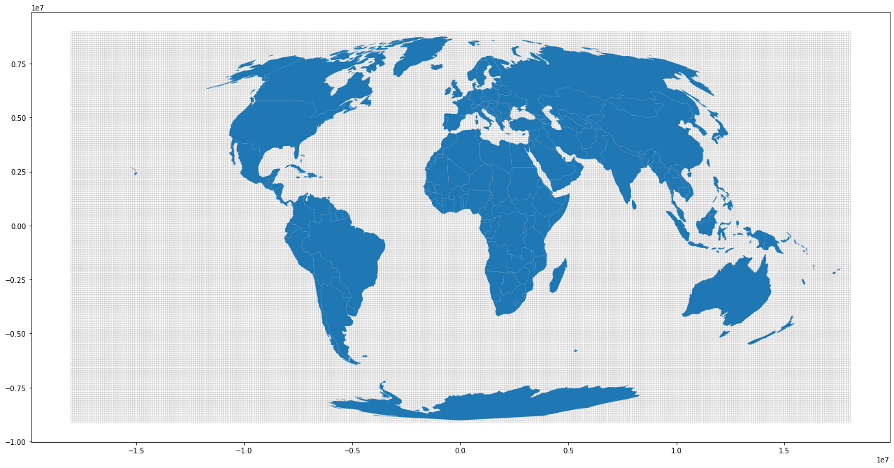
Preview Grid
base = grid.plot(figsize=(22,28), color='white', edgecolor='black', linewidth=0.1)
# combine with world geometry
plot = world.plot(ax=base)
Prepare binary search
The aggregation speed is important here and we should not use polygon intersection. Since we're working with a regular grid and floating point numbers, a binary search is likely one of the fastest ways for our context. numpy.digitize provides a binary search, but it must be adapted to for the spatial context. A lat or lng value is assigned to the nearest bin matching. We get our lat and lng bins from our original Mollweide grid, which are regularly spaced at 100km interval. Note that we need to do two binary searches, for lat and for lng values.
Create test points
testpoint = Point(8.546377, 47.392323)
testpoint2 = Point(13.726359, 51.028512)
gdf_testpoints = gp.GeoSeries([testpoint, testpoint2], crs=crs_wgs)
# project geometries to Mollweide
gdf_testpoints_proj = gdf_testpoints.to_crs(crs_proj)
gdf_testpoints_proj[0].x
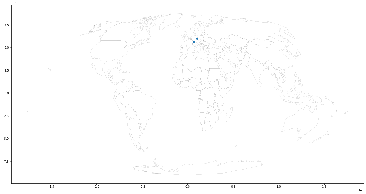
Preview map for testpoint
base = world.plot(figsize=(22,28), color='white', edgecolor='black', linewidth=0.1)
plot = gdf_testpoints_proj.plot(ax=base)
Use np.digitize() to assign coordinates to the grid
np.digitize is implemented in terms of np.searchsorted. This means that a binary search is used to bin the values, which scales much better for larger number of bins than the previous linear search. It also removes the requirement for the input array to be 1-dimensional.
Create 2 bins for each axis of existing Mollweide rows/cols grid:
ybins = np.array(rows)
xbins = np.array(cols)
Create 2 lists with a single entry (testpoint coordinate)
test_point_list_x = np.array([gdf_testpoints_proj[0].x, gdf_testpoints_proj[1].x])
test_point_list_y = np.array([gdf_testpoints_proj[0].y, gdf_testpoints_proj[1].y])
Find the nearest bin for x coordinate (returns the bin-index):
x_bin = np.digitize(test_point_list_x, xbins) - 1
display(x_bin)
Check value of bin (the y coordinate) based on returned index:
testpoint_xbin_idx = xbins[[x_bin[0], x_bin[1]]]
display(testpoint_xbin_idx)
Repeat the same for y-testpoint:
y_bin = np.digitize(test_point_list_y, ybins) - 1
display(y_bin)
testpoint_ybin_idx = ybins[[y_bin[0], y_bin[1]]]
display(testpoint_ybin_idx)
➡️ 759904 / 5579952 and 1059904 / 5979952 are indexes that we can use in our geodataframe index to return the matching grid-poly for each point
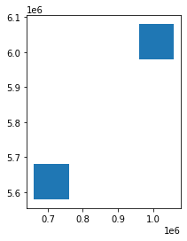
Highlight Testpoint in Grid
Get grid-poly by index from testpoint
grid.loc[testpoint_xbin_idx[0], testpoint_ybin_idx[0]]
Convert shapely bin poly to Geoseries and plot
testpoint_grids = gp.GeoSeries([grid.loc[testpoint_xbin_idx[0], testpoint_ybin_idx[0]].geometry, grid.loc[testpoint_xbin_idx[1], testpoint_ybin_idx[1]].geometry])
testpoint_grids.plot()
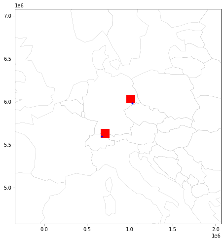
Preview map with testpoint and assigned bin
Set auto zoom with buffer:
minx, miny, maxx, maxy = testpoint_grids.total_bounds
buf = 1000000
# a figure with a 1x1 grid of Axes
fig, ax = plt.subplots(1, 1,figsize=(10,8))
ax.set_xlim(minx-buf, maxx+buf)
ax.set_ylim(miny-buf, maxy+buf)
base = world.plot(ax=ax, color='white', edgecolor='black', linewidth=0.1)
grid_base = testpoint_grids.plot(ax=base, facecolor='red', linewidth=0.1)
plot = gdf_testpoints_proj.plot(ax=grid_base, markersize=8, color='blue')
Prepare functions
Now that it has been visually verified that the algorithm works, lets create functions for the main processing job.
def get_best_bins(
    search_values_x: np.array, search_values_y: np.array,
    xbins: np.array, ybins: np.array) -> Tuple[np.ndarray, np.ndarray]:
    """Will return best bin for a lat and lng input

    Note: prepare bins and values in correct matching projection

    Args:
        search_values_y: A list of projected latitude values
        search_values_x: A list of projected longitude values
        xbins: 1-d array of bins to snap lat/lng values
        ybins: 1-d array of bins to snap lat/lng values

    Returns:
        Tuple[int, int]: A list of tuples with 2 index positions for the best
            matching bins for each lat/lng
    """
    xbins_idx = np.digitize(search_values_x, xbins, right=False)
    ybins_idx = np.digitize(search_values_y, ybins, right=False)
    return (xbins[xbins_idx-1], ybins[ybins_idx-1])
Test with LBSN data
We're going to test the binning of coordinates on a part of the YFCC geotagged images.
Prepare lat/lng tuple of lower left corner and upper right corner to crop sample map:
# Part of Italy and Sicily
bbox_italy = (
    7.8662109375, 36.24427318493909,
    19.31396484375, 43.29320031385282)
bbox = bbox_italy
Calculate bounding box with 1000 km buffer. For that, project the bounding Box to Mollweide, apply the buffer, and project back to WGS1984:
#convert to Mollweide
minx, miny = proj_transformer.transform(
    bbox_italy[0], bbox_italy[1])
maxx, maxy = proj_transformer.transform(
    bbox_italy[2], bbox_italy[3])
# apply buffer and convetr back to WGS1984
min_buf = proj_transformer_back.transform(minx-buf, miny-buf)
max_buf = proj_transformer_back.transform(maxx+buf, maxy+buf)
bbox_italy_buf = [min_buf[0], min_buf[1], max_buf[0], max_buf[1]]
Select columns and types for improving speed
usecols = ['latitude', 'longitude', 'post_hll']
dtypes = {'latitude': float, 'longitude': float}
reset_metrics(grid, metrics)
Load data
%%time
df = pd.read_csv(
    "yfcc_latlng.csv", usecols=usecols, dtype=dtypes, encoding='utf-8')
print(len(df))
Filter on bounding box (Italy)
def filter_df_bbox(
    df: pd.DataFrame, bbox: Tuple[float, float, float, float],
    inplace: bool = True):
    """Filter dataframe with bbox on latitude and longitude column"""
    df.query(
        f'({bbox_italy_buf[0]} < longitude) & '
        f'(longitude <  {bbox_italy_buf[2]}) & '
        f'({bbox_italy_buf[1]} < latitude) & '
        f'(latitude < {bbox_italy_buf[3]})',
        inplace=True)
    # set index to asc integers
    if inplace:
        df.reset_index(inplace=True, drop=True)
        return
    return df.reset_index(inplace=False, drop=True)
Execute and count number of posts in the bounding box:
%%time
filter_df_bbox(df=df, bbox=bbox_italy_buf)
print(f"There're {len(df):,.0f} YFCC distinct lat-lng coordinates located within the bounding box.")
df.head()
Project coordinates to Mollweide
Projection speed can be increased by using a predefined pyproj.Transformer. We're also splitting our input-dataframe into a list of dataframe, each containing 1 Million records, so we can process the data in chunks.
def proj_df(df, proj_transformer):
    """Project pandas dataframe latitude and longitude decimal degrees
    using predefined proj_transformer"""
    if 'longitude' not in df.columns:
        return
    xx, yy = proj_transformer.transform(
        df['longitude'].values, df['latitude'].values)
    # assign projected coordinates to
    # new columns x and y
    # the ':' means: replace all values in-place
    df.loc[:, "x"] = xx
    df.loc[:, "y"] = yy
    # Drop WGS coordinates
    df.drop(columns=['longitude', 'latitude'], inplace=True)
%%time
proj_df(df, proj_transformer)
print(f'Projected {len(df.values)} coordinates')
df.head()
Perform the bin assignment
%%time
xbins_match, ybins_match = get_best_bins(
    search_values_x=df['x'].to_numpy(),
    search_values_y=df['y'].to_numpy(),
    xbins=xbins, ybins=ybins)
len(xbins_match)
xbins_match[:10]
ybins_match[:10]
A: Estimated Post Count per grid
Attach target bins to original dataframe. The : means: modify all values in-place
df.loc[:, 'xbins_match'] = xbins_match
df.loc[:, 'ybins_match'] = ybins_match
# set new index column
df.set_index(['xbins_match', 'ybins_match'], inplace=True)
# drop x and y columns not needed anymore
df.drop(columns=['x', 'y'], inplace=True)
df.head()
The next step is to union hll sets and (optionally) return the cardinality (the number of distinct elements). This can only be done by connecting to a postgres database with HLL extension installed. We're using our hlldb here, but it is equally possible to connect to an empty Postgres DB such as pg-hll-empty docker container.
def union_hll(
    hll_series: pd.Series, cardinality: bool = True) -> pd.Series:
    """HLL Union and (optional) cardinality estimation from series of hll sets
    based on group by composite index.

        Args:
        hll_series: Indexed series (bins) of hll sets.
        cardinality: If True, returns cardinality (counts). Otherwise,
            the unioned hll set will be returned.

    The method will combine all groups of hll sets first,
        in a single SQL command. Union of hll hll-sets belonging
        to the same group (bin) and (optionally) returning the cardinality
        (the estimated count) per group will be done in postgres.

    By utilizing Postgres´ GROUP BY (instead of, e.g. doing
        the group with numpy), it is possible to reduce the number
        of SQL calls to a single run, which saves overhead
        (establishing the db connection, initializing the SQL query
        etc.). Also note that ascending integers are used for groups,
        instead of their full original bin-ids, which also reduces
        transfer time.

    cardinality = True should be used when calculating counts in
        a single pass.

    cardinality = False should be used when incrementally union
        of hll sets is required, e.g. due to size of input data.
        In the last run, set to cardinality = True.
    """
    # group all hll-sets per index (bin-id)
    series_grouped = hll_series.groupby(
        hll_series.index).apply(list)
    # From grouped hll-sets,
    # construct a single SQL Value list;
    # if the following nested list comprehension
    # doesn't make sense to you, have a look at
    # spapas.github.io/2016/04/27/python-nested-list-comprehensions/
    # with a decription on how to 'unnest'
    # nested list comprehensions to regular for-loops
    hll_values_list = ",".join(
        [f"({ix}::int,'{hll_item}'::hll)"
         for ix, hll_items
         in enumerate(series_grouped.values.tolist())
         for hll_item in hll_items])
    # Compilation of SQL query,
    # depending on whether to return the cardinality
    # of unioned hll or the unioned hll
    return_col = "hll_union"
    hll_calc_pre = ""
    hll_calc_tail = "AS hll_union"
    if cardinality:
        # add sql syntax for cardinality
        # estimation
        # (get count distinct from hll)
        return_col = "hll_cardinality"
        hll_calc_pre = "hll_cardinality("
        hll_calc_tail = ")::int"
    db_query = f"""
        SELECT sq.{return_col} FROM (
            SELECT s.group_ix,
                   {hll_calc_pre}
                   hll_union_agg(s.hll_set)
                   {hll_calc_tail}
            FROM (
                VALUES {hll_values_list}
                ) s(group_ix, hll_set)
            GROUP BY group_ix
            ORDER BY group_ix ASC) sq
        """
    df = db_conn.query(db_query)
    # to merge values back to grouped dataframe,
    # first reset index to ascending integers
    # matching those of the returned df;
    # this will turn series_grouped into a DataFrame;
    # the previous index will still exist in column 'index'
    df_grouped = series_grouped.reset_index()
    # drop hll sets not needed anymore
    df_grouped.drop(columns=[hll_series.name], inplace=True)
    # append hll_cardinality counts
    # using matching ascending integer indexes
    df_grouped.loc[df.index, return_col] = df[return_col]
    # set index back to original bin-ids
    df_grouped.set_index("index", inplace=True)
    # split tuple index to produce
    # the multiindex of the original dataframe
    # with xbin and ybin column names
    df_grouped.index = pd.MultiIndex.from_tuples(
        df_grouped.index, names=['xbin', 'ybin'])
    # return column as indexed pd.Series
    return df_grouped[return_col]
Optionally, split dataframe into chunks, so we're not the exceeding memory limit (e.g. use if memory < 16GB). A chunk size of 1 Million records is suitable for a computer with about 8 GB of memory and optional sparse HLL mode enabled. If sparse mode is disabled, decrease chunk_size accordingly, to compensate for increased space.
%%time
chunked_df = [
    df[i:i+CHUNK_SIZE] for i in range(0, df.shape[0], CHUNK_SIZE)]
chunked_df[0].head()
To test, process the first chunk:
%%time
cardinality_series = union_hll(chunked_df[0]["post_hll"])
cardinality_series.head()
Remove possibly existing result column in grid from previous run:
reset_metrics(grid, ["postcount_est"], setzero=True)
Append Series with calculated counts to grid (as new column) based on index match:
grid.loc[cardinality_series.index, 'postcount_est'] = cardinality_series
grid[grid["postcount_est"] > 0].head()
Process all chunks:
The caveat here is to incrementally union hll sets until all records have been processed. On the last loop, instruct the hll worker to return the cardinality instead of the unioned hll set.
First, define method to join cardinality to grid
# reference metric names and column names
column_metric_ref = {
        "postcount_est":"post_hll",
        "usercount_est":"user_hll",
        "userdays_est":"date_hll"}

def join_df_grid(
    df: pd.DataFrame, grid: gp.GeoDataFrame,
    metric: str = "postcount_est",
    cardinality: bool = True):
    """Union HLL Sets and estimate postcount per
    grid bin from lat/lng coordinates

        Args:
        df: A pandas dataframe with latitude and
            longitude columns in WGS1984
        grid: A geopandas geodataframe with indexes
            x and y (projected coordinates) and grid polys
        metric: target column for estimate aggregate.
            Default: postcount_est.
        cardinality: will compute cardinality of unioned
            hll sets. Otherwise, unioned hll sets will be
            returned for incremental updates.
    """
    # optionally, bin assigment of projected coordinates,
    # make sure to not bin twice:
    # x/y columns are removed after binning
    if 'x' in df.columns:
        bin_coordinates(df, xbins, ybins)
        # set index column
        df.set_index(
            ['xbins_match', 'ybins_match'], inplace=True)
    # union hll sets and
    # optional estimate count distincts (cardinality)
    column = column_metric_ref.get(metric)
    # get series with grouped hll sets
    hll_series = df[column]
    # union of hll sets:
    # to allow incremental union of already merged data
    # and new data, concatenate series from grid and new df
    # only if column with previous hll sets already exists
    if metric in grid.columns:
        # remove nan values from grid and
        # rename series to match names
        hll_series = pd.concat(
            [hll_series, grid[metric].dropna()]
            ).rename(column)
    cardinality_series = union_hll(
        hll_series, cardinality=cardinality)
    # add unioned hll sets/computed cardinality to grid
    grid.loc[
        cardinality_series.index, metric] = cardinality_series
    if cardinality:
        # set all remaining grid cells
        # with no data to zero and
        # downcast column type from float to int
        grid[metric] = grid[metric].fillna(0).astype(int)
Define method to process chunks:
def join_chunkeddf_grid(
    chunked_df: List[pd.DataFrame], grid: gp.GeoDataFrame,
    metric: str = "postcount_est", chunk_size: int = CHUNK_SIZE,
    benchmark_data: Optional[bool] = None):
    """Incremental union of HLL Sets and estimate postcount per
    grid bin from chunked list of dataframe records. Results will
    be stored in grid.

    Args:
    chunked_df: A list of (chunked) dataframes with latitude and
        longitude columns in WGS1984
    grid: A geopandas geodataframe with indexes
        x and y (projected coordinates) and grid polys
    metric: target column for estimate aggregate.
        Default: postcount_est.
    benchmark_data: If True, will not remove HLL sketches after
        final cardinality estimation.
    """
    reset_metrics(grid, [metric])
    for ix, chunk_df in enumerate(chunked_df):
        # compute cardinality only on last iteration
        cardinality = False
        if ix == len(chunked_df)-1:
            cardinality = True
        column = column_metric_ref.get(metric)
        # get series with grouped hll sets
        hll_series = chunk_df[column]
        if metric in grid.columns:
            # merge existing hll sets with new ones
            # into one series (with duplicate indexes);
            # remove nan values from grid and
            # rename series to match names
            hll_series = pd.concat(
                [hll_series, grid[metric].dropna()]
                ).rename(column)
        cardinality_series = union_hll(
            hll_series, cardinality=cardinality)
        if benchmark_data:
            # only if final hll sketches need to
            # be kept for benchmarking:
            # do another union, without cardinality
            # estimation, and store results
            # in column "metric"_hll
            hll_sketch_series = union_hll(
                hll_series, cardinality=False)
            grid.loc[
                hll_sketch_series.index,
                f'{metric.replace("_est","_hll")}'] = hll_sketch_series
        # add unioned hll sets/computed cardinality to grid
        grid.loc[
            cardinality_series.index, metric] = cardinality_series
        if cardinality:
            # set all remaining grid cells
            # with no data to zero and
            # downcast column type from float to int
            grid[metric] = grid[metric].fillna(0).astype(int)
        clear_output(wait=True)
        print(f'Mapped ~{(ix+1)*chunk_size} coordinates to bins')
join_chunkeddf_grid(chunked_df, grid, chunk_size=CHUNK_SIZE)
All distinct counts are now attached to the bins of the grid:
grid[grid["postcount_est"]>10].head()
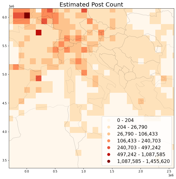
Preview post count map
# create bounds from WGS1984 italy and project to Mollweide
minx, miny = proj_transformer.transform(
    bbox_italy[0], bbox_italy[1])
maxx, maxy = proj_transformer.transform(
    bbox_italy[2], bbox_italy[3])
Use headtail_breaks classification scheme because it is specifically suited to map long tailed data, see Jiang 2013
- Jiang, B. (August 01, 2013). Head/Tail Breaks: A New Classification Scheme for Data with a Heavy-Tailed Distribution. The Professional Geographer, 65, 3, 482-494.
# global legend font size setting
plt.rc('legend', **{'fontsize': 16})

def leg_format(leg):
    "Format matplotlib legend entries"
    for lbl in leg.get_texts():
        label_text = lbl.get_text()
        lower = label_text.split()[0]
        upper = label_text.split()[2]
        new_text = f'{float(lower):,.0f} - {float(upper):,.0f}'
        lbl.set_text(new_text)

def title_savefig_mod(title, save_fig):
    """Update title/output name if grid size is not 100km"""
    if GRID_SIZE_METERS == 100000:
        return title, save_fig
    km_size = GRID_SIZE_METERS/1000
    title = f'{title} ({km_size:.0f}km grid)'
    if save_fig:
        save_fig = save_fig.replace(
            '.png', f'_{km_size:.0f}km.png')
    return title, save_fig

def save_plot(
    grid: gp.GeoDataFrame, title: str, column: str, save_fig: str = None):
    """Plot GeoDataFrame with matplotlib backend, optionaly export as png"""
    fig, ax = plt.subplots(1, 1,figsize=(10,12))
    ax.set_xlim(minx-buf, maxx+buf)
    ax.set_ylim(miny-buf, maxy+buf)
    title, save_fig = title_savefig_mod(
        title, save_fig)
    ax.set_title(title, fontsize=20)
    base = grid.plot(
        ax=ax, column=column, cmap='OrRd', scheme='headtail_breaks',
        legend=True, legend_kwds={'loc': 'lower right'})
    # combine with world geometry
    plot = world.plot(
        ax=base, color='none', edgecolor='black', linewidth=0.1)
    leg = ax.get_legend()
    leg_format(leg)
    if not save_fig:
        return
    fig.savefig(Path("OUT") / save_fig, dpi=300, format='PNG',
                bbox_inches='tight', pad_inches=1)
save_plot(
    grid=grid, title='Estimated Post Count',
    column='postcount_est', save_fig='postcount_sample_est.png')
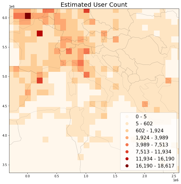
B: Estimated User Count per grid
When using HLL, aggregation of user_guids or user_days takes the same amount of time (unlike when working with original data, where memory consumption increases significantly). We'll only need to update the columns that are loaded from the database:
usecols = ['latitude', 'longitude', 'user_hll']
Adjust method for stream-reading from CSV in chunks:
iter_csv = pd.read_csv(
    "yfcc_latlng.csv", usecols=usecols, iterator=True,
    dtype=dtypes, encoding='utf-8', chunksize=CHUNK_SIZE)
def proj_report(df, proj_transformer, cnt, inplace: bool = False):
    """Project df with progress report"""
    proj_df(df, proj_transformer)
    clear_output(wait=True)
    print(f'Projected {cnt:,.0f} coordinates')
    if inplace:
        return
    return df
%%time
# filter
chunked_df = [
    filter_df_bbox(
        df=chunk_df, bbox=bbox_italy_buf, inplace=False)
    for chunk_df in iter_csv]

# project
projected_cnt = 0
for chunk_df in chunked_df:
    projected_cnt += len(chunk_df)
    proj_report(
        chunk_df, proj_transformer, projected_cnt, inplace=True)

chunked_df[0].head()
Perform the bin assignment and estimate distinct users
def bin_coordinates(
        df: pd.DataFrame, xbins:
        np.ndarray, ybins: np.ndarray) -> pd.DataFrame:
    """Bin coordinates using binary search and append to df as new index"""
    xbins_match, ybins_match = get_best_bins(
        search_values_x=df['x'].to_numpy(),
        search_values_y=df['y'].to_numpy(),
        xbins=xbins, ybins=ybins)
    # append target bins to original dataframe
    # use .loc to avoid chained indexing
    df.loc[:, 'xbins_match'] = xbins_match
    df.loc[:, 'ybins_match'] = ybins_match
    # drop x and y columns not needed anymore
    df.drop(columns=['x', 'y'], inplace=True)
def bin_chunked_coordinates(
    chunked_df: List[pd.DataFrame]):
    """Bin coordinates of chunked dataframe"""
    binned_cnt = 0
    for ix, df in enumerate(chunked_df):
        bin_coordinates(df, xbins, ybins)
        df.set_index(['xbins_match', 'ybins_match'], inplace=True)
        clear_output(wait=True)
        binned_cnt += len(df)
        print(f"Binned {binned_cnt:,.0f} coordinates..")
%%time
bin_chunked_coordinates(chunked_df)
chunked_df[0].head()
Union HLL Sets per grid-id and calculate cardinality (estimated distinct user count):
join_chunkeddf_grid(
    chunked_df=chunked_df, grid=grid, metric="usercount_est")
grid[grid["usercount_est"]> 0].head()
Look at this. There're many polygons were thounsands of photos have been created by only few users. Lets see how this affects our test map..
Preview user count map
save_plot(
    grid=grid, title='Estimated User Count',
    column='usercount_est', save_fig='usercount_sample_est.png')
C: Estimated User Days
The sequence of commands for userdays is exactly the same as for postcount and usercount above.
usecols = ['latitude', 'longitude', 'date_hll']
def read_project_chunked(filename: str,
    usecols: List[str], chunk_size: int = CHUNK_SIZE,
    bbox: Tuple[float, float, float, float] = None) -> List[pd.DataFrame]:
    """Read data from csv, optionally clip to bbox and projet"""
    iter_csv = pd.read_csv(
        filename, usecols=usecols, iterator=True,
        dtype=dtypes, encoding='utf-8', chunksize=chunk_size)
    if bbox:
        chunked_df = [filter_df_bbox(
            df=chunk_df, bbox=bbox, inplace=False)
        for chunk_df in iter_csv]
    else:
        chunked_df = [chunk_df for chunk_df in iter_csv]
    # project
    projected_cnt = 0
    for chunk_df in chunked_df:
        projected_cnt += len(chunk_df)
        proj_report(
            chunk_df, proj_transformer, projected_cnt, inplace=True)
    return chunked_df
Run:
%%time
chunked_df = read_project_chunked(
    filename="yfcc_latlng.csv",
    usecols=usecols,
    bbox=bbox_italy_buf)
chunked_df[0].head()
%%time
bin_chunked_coordinates(chunked_df)
join_chunkeddf_grid(
    chunked_df=chunked_df, grid=grid, metric="userdays_est")
chunked_df[0].head()
grid[grid["userdays_est"]> 0].head()
save_plot(
    grid=grid, title='Estimated User Days',
    column='userdays_est', save_fig='userdays_sample_est.png')
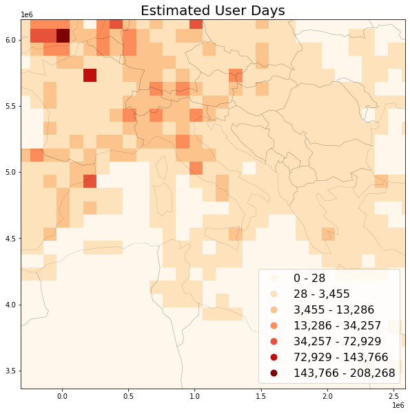
There're other approaches for further reducing noise. For example, to reduce the impact of automatic capturing devices (such as webcams uploading x pictures per day), a possibility is to count distinct userlocations. For userlocations metric, a user would be counted multiple times per grid bin only for pictures with different lat/lng. Or the number of distinct userlocationdays (etc.). These metrics easy to implement using hll, but would be quite difficult to compute using raw data.
Prepare methods
Lets summarize the above code in a few methods:
Plotting preparation
The below methods contain combined code from above, plus final plot style improvements.
def format_legend(
    leg, bounds: List[str], inverse: bool = None,
    metric: str = "postcount_est"):
    """Formats legend (numbers rounded, colors etc.)"""
    leg.set_bbox_to_anchor((0., 0.2, 0.2, 0.2))
    # get all the legend labels
    legend_labels = leg.get_texts()
    plt.setp(legend_labels, fontsize='12')
    lcolor = 'black'
    if inverse:
        frame = leg.get_frame()
        frame.set_facecolor('black')
        frame.set_edgecolor('grey')
        lcolor = "white"
    plt.setp(legend_labels, color = lcolor)
    if metric == "postcount_est":
        leg.set_title("Estimated Post Count")
    elif metric == "usercount_est":
        leg.set_title("Estimated User Count")
    else:
        leg.set_title("Estimated User Days")
    plt.setp(leg.get_title(), fontsize='12')
    leg.get_title().set_color(lcolor)
    # replace the numerical legend labels
    for bound, legend_label in zip(bounds, legend_labels):
        legend_label.set_text(bound)
def format_bound(
    upper_bound: float = None, lower_bound: float = None) -> str:
    """Format legend text for class bounds"""
    if upper_bound is None:
        return f'{lower_bound:,.0f}'
    if lower_bound is None:
        return f'{upper_bound:,.0f}'
    return f'{lower_bound:,.0f} - {upper_bound:,.0f}'

def get_label_bounds(
    scheme_classes, metric_series: pd.Series,
    flat: bool = None) -> List[str]:
    """Get all upper bounds in the scheme_classes category"""
    upper_bounds = scheme_classes.bins
    # get and format all bounds
    bounds = []
    for idx, upper_bound in enumerate(upper_bounds):
        if idx == 0:
            lower_bound = metric_series.min()
        else:
            lower_bound = upper_bounds[idx-1]
        if flat:
            bound = format_bound(
                lower_bound=lower_bound)
        else:
            bound = format_bound(
                upper_bound, lower_bound)
        bounds.append(bound)
    if flat:
        upper_bound = format_bound(
            upper_bound=upper_bounds[-1])
        bounds.append(upper_bound)
    return bounds

def label_nodata(
    grid: gp.GeoDataFrame, inverse: bool = None,
    metric: str = "postcount_est"):
    """Add white to a colormap to represent missing value

    Adapted from:
        https://stackoverflow.com/a/58160985/4556479

    See available colormaps:
        http://holoviews.org/user_guide/Colormaps.html
    """
    # set 0 to NaN
    grid_nan = grid[metric].replace(0, np.nan)
    # get headtail_breaks
    # excluding NaN values
    headtail_breaks = mc.HeadTailBreaks(
        grid_nan.dropna())
    grid[f'{metric}_cat'] = headtail_breaks.find_bin(
        grid_nan).astype('str')
    # set label for NaN values
    grid.loc[grid_nan.isnull(), f'{metric}_cat'] = 'No Data'
    bounds = get_label_bounds(
        headtail_breaks, grid_nan.dropna().values)
    cmap_name = 'OrRd'
    nodata_color = 'white'
    if inverse:
        nodata_color = 'black'
        cmap_name = 'fire'
    cmap = plt.cm.get_cmap(cmap_name, headtail_breaks.k)
    # get hex values
    cmap_list = [colors.rgb2hex(cmap(i)) for i in range(cmap.N)]
    # lighten or darken up first/last color a bit
    # to offset from black or white background
    if inverse:
        firstcolor = '#3E0100'
        cmap_list[0] = firstcolor
    else:
        lastcolor = '#440402'
        cmap_list.append(lastcolor)
        cmap_list.pop(0)
    # append nodata color
    cmap_list.append(nodata_color)
    cmap_with_nodata = colors.ListedColormap(cmap_list)
    return cmap_with_nodata, bounds

def plot_figure(
    grid: gp.GeoDataFrame, title: str, inverse: bool = None,
    metric: str = "postcount_est", store_fig: str = None):
    """Combine layers and plot"""
    # for plotting, there're some minor changes applied
    # to the dataframe (replace NaN values),
    # make a shallow copy here to prevent changes
    # to modify the original grid
    grid_plot = grid.copy()
    # create new plot figure object with one axis
    fig, ax = plt.subplots(1, 1, figsize=(22,28))
    ax.set_title(title, fontsize=16)
    print("Classifying bins..")
    cmap_with_nodata, bounds = label_nodata(
        grid=grid_plot, inverse=inverse, metric=metric)
    base = grid_plot.plot(
        ax=ax,
        column=f'{metric}_cat', cmap=cmap_with_nodata, legend=True)
    print("Formatting legend..")
    leg = ax.get_legend()
    format_legend(leg, bounds, inverse, metric)
    # combine with world geometry
    edgecolor = 'black'
    if inverse:
        edgecolor = 'white'
    plot = world.plot(
        ax=base, color='none', edgecolor=edgecolor, linewidth=0.1)
    if store_fig:
        print("Storing figure as png..")
        if inverse:
            store_fig = store_fig.replace('.png', '_inverse.png')
        fig.savefig(
            Path("OUT") / store_fig, dpi=300, format='PNG',
            bbox_inches='tight', pad_inches=1)
def load_plot(
    grid: gp.GeoDataFrame, title: str, inverse: bool = None,
    metric: str = "postcount_est", store_fig: str = None, store_pickle: str = None,
    chunk_size: int = CHUNK_SIZE, benchmark_data: Optional[bool] = None):
    """Load data, bin coordinates, estimate distinct counts (cardinality) and plot map

        Args:
        data: Path to read input CSV
        grid: A geopandas geodataframe with indexes x and y
            (projected coordinates) and grid polys
        title: Title of the plot
        inverse: If True, inverse colors (black instead of white map)
        metric: target column for aggregate. Default: postcount_est.
        store_fig: Provide a name to store figure as PNG. Will append
            '_inverse.png' if inverse=True.
        store_pickle: Provide a name to store pickled dataframe
            with aggregate counts to disk
        chunk_size: chunk processing into x records per chunk
        benchmark_data: If True, hll_sketches will not be removed
            after final estimation of cardinality
    """
    usecols = ['latitude', 'longitude']
    column = column_metric_ref.get(metric)
    usecols.append(column)
    # get data from csv
    chunked_df = read_project_chunked(
        filename="yfcc_latlng.csv",
        usecols=usecols)
    # bin coordinates
    bin_chunked_coordinates(chunked_df)
    # reset metric column
    reset_metrics(grid, [metric], setzero=False)
    print("Getting cardinality per bin..")
    # union hll sets per chunk and
    # calculate distinct counts on last iteration
    join_chunkeddf_grid(
        chunked_df=chunked_df, grid=grid,
        metric=metric, chunk_size=chunk_size,
        benchmark_data=benchmark_data)
    # store intermediate data
    if store_pickle:
        print("Storing aggregate data as pickle..")
        grid.to_pickle(store_pickle)
    print("Plotting figure..")
    plot_figure(grid, title, inverse, metric, store_fig)
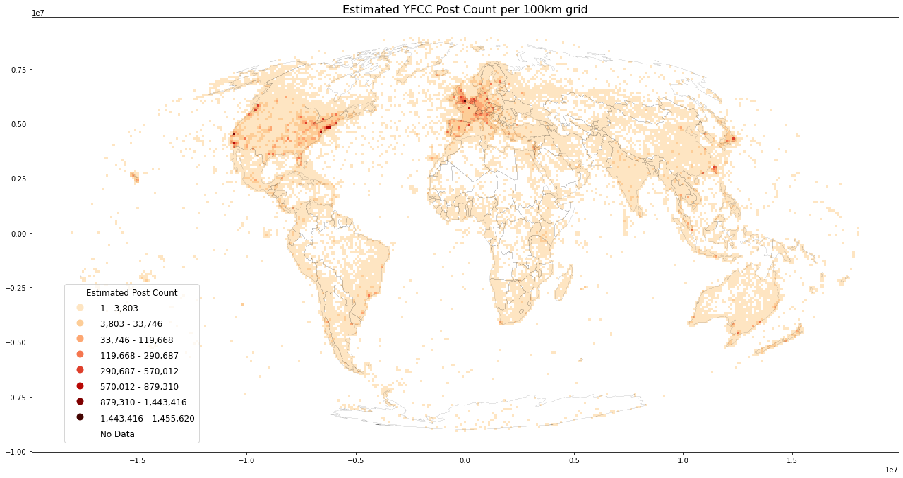
Plotting worldmaps: Post Count, User Count and User Days
Plot worldmap for each datasource
reset_metrics(grid, ["postcount_est", "usercount_est", "userdays_est"])
%%time
%%memit
load_plot(
    grid, title=f'Estimated YFCC Post Count per {int(length/1000)}km grid',
    inverse=False, store_fig="yfcc_postcount_est.png", benchmark_data=True)
%%time
%%memit
load_plot(
    grid, title=f'Estimated YFCC User Count per {int(length/1000)}km grid',
    inverse=False, store_fig="yfcc_usercount_est.png",
    metric="usercount_est", benchmark_data=True)
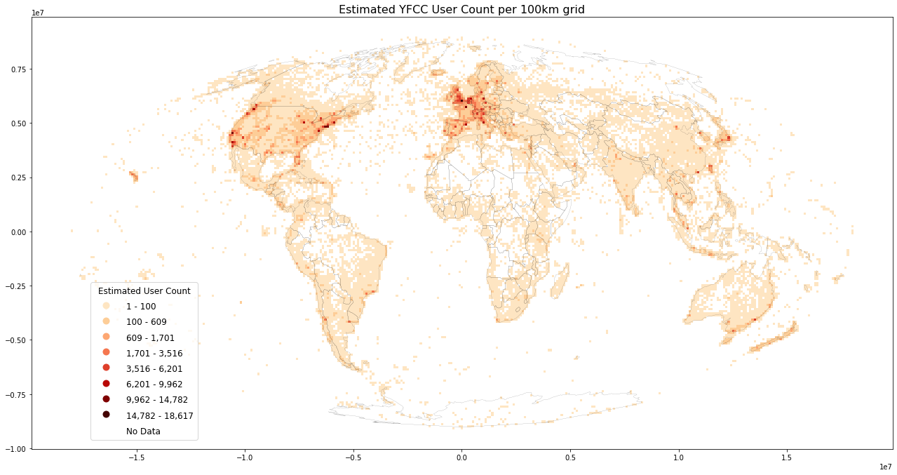
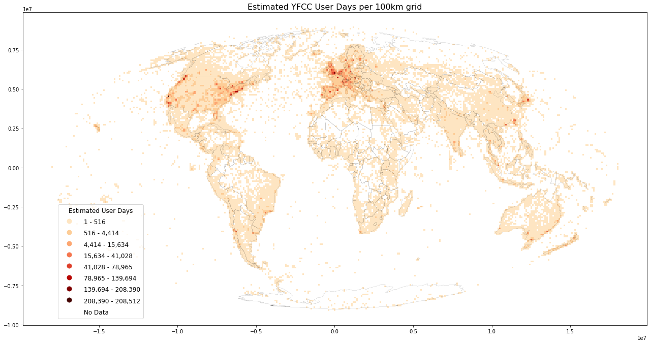
%%time
%%memit
load_plot(
    grid, title=f'Estimated YFCC User Days per {int(length/1000)}km grid',
    inverse=False, store_fig="yfcc_userdays_est.png",
    metric="userdays_est", benchmark_data=True)
Have a look at the final grid with estimated cardinality for postcount, usercount and userdays
We can make an immediate validation of the numbers by verifying that postcount >= userdays >= usercount. On very rare occasions and edge cases, this may invalidate due to the estimation error of 3 to 5% of HyperLogLog derived cardinality.
grid[grid["postcount_est"]>1].drop(
    ['geometry', 'usercount_hll', 'postcount_hll', 'userdays_hll'], axis=1, errors="ignore").head()
Final HLL Sets are also available, as benchmark data, in columns usercount_hll, postcount_hll, userdays_hll columns:
grid[grid["postcount_est"]>1].drop(
    ['geometry', 'usercount_est', 'postcount_est', 'userdays_est'], axis=1, errors="ignore").head()
Store results to CSV for archive purposes:
Define method
def grid_agg_tocsv(
    grid: gp.GeoDataFrame, filename: str,
    metrics: List[str] = ["postcount_est", "usercount_est", "userdays_est"]):
    """Store geodataframe aggregate columns and indexes to CSV"""
    grid.to_csv(filename, mode='w', columns=metrics, index=True)
Convert/store to CSV (aggregate columns and indexes only):
grid_agg_tocsv(grid, "yfcc_all_est.csv")
Store results as benchmark data (with hll sketches):
As a minimal protection against intersection attacks on published data, only export hll sets with cardinality > 1000.
grid_agg_tocsv(
    grid[grid["usercount_est"]>100], "yfcc_all_est_benchmark.csv",
    metrics = ["postcount_est", "usercount_est", "userdays_est",
               "usercount_hll", "postcount_hll", "userdays_hll"])
Size of benchmark data:
benchmark_size_mb = Path("yfcc_all_est_benchmark.csv").stat().st_size / (1024*1024)
print(f"Size: {benchmark_size_mb:.2f} MB")
Load data from CSV:
def create_new_grid(
    length: int = GRID_SIZE_METERS, width: int = GRID_SIZE_METERS) -> gp.GeoDataFrame:
    """Create new 100x100km grid GeoDataFrame (Mollweide)"""
    # Mollweide projection epsg code
    epsg_code = 54009
    crs_proj = f"esri:{epsg_code}"
    crs_wgs = "epsg:4326"
    # define Transformer ahead of time
    # with xy-order of coordinates
    proj_transformer = Transformer.from_crs(
        crs_wgs, crs_proj, always_xy=True)
    # grid bounds from WGS1984 to Mollweide
    xmin = proj_transformer.transform(
        -180, 0)[0]
    xmax = proj_transformer.transform(
        180, 0)[0]
    ymax = proj_transformer.transform(
        0, 90)[1]
    ymin = proj_transformer.transform(
        0, -90)[1]
    # define grid size
    length = length
    width = width
    grid = create_grid_df(
        length=length, width=width,
        xmin=xmin, ymin=ymin,
        xmax=xmax, ymax=ymax)
    # convert grid DataFrame to grid GeoDataFrame
    grid = grid_to_gdf(grid)
    return grid

def grid_agg_fromcsv(
    filename: str, metrics: List[str] = ["postcount_est", "usercount_est"],
    length: int = GRID_SIZE_METERS, width: int = GRID_SIZE_METERS):
    """Create a new Mollweide grid GeoDataFrame and
    attach aggregate data columns from CSV based on index"""
    # 1. Create new 100x100km (e.g.) grid
    grid = create_new_grid(length=length, width=width)
    # 2. load aggregate data from CSV and attach to grid
    # -----
    types_dict = dict()
    for metric in metrics:
        types_dict[metric] = int
    df = pd.read_csv(
        filename, dtype=types_dict, index_col=["xbin", "ybin"])
    # join columns based on index
    grid = grid.join(df)
    # return grid with aggregate data attached
    return grid
To create a new grid and load aggregate counts from CSV:
grid = grid_agg_fromcsv(
    "yfcc_all_est.csv", length=length, width=width)
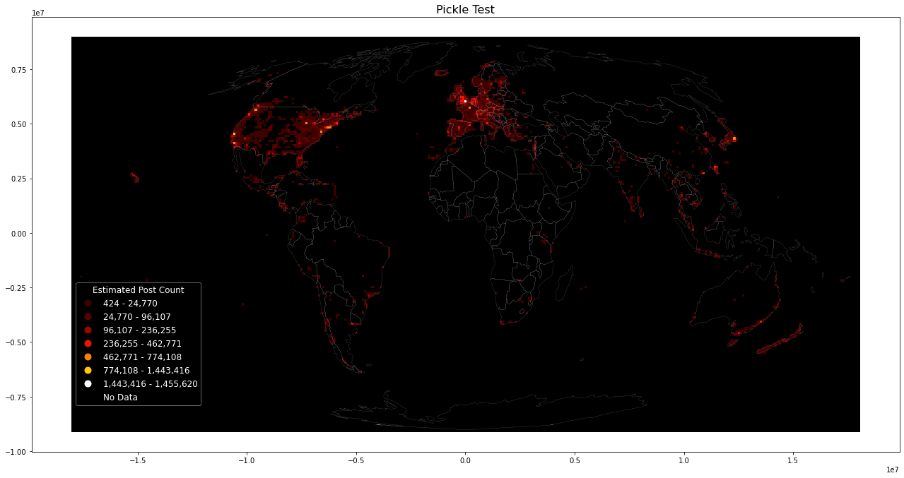
Load & plot pickled dataframe
Loading (geodataframe) using pickle. This is the easiest way to store intermediate data, but may be incompatible if package versions change. If loading pickles does not work, a workaround is to load data from CSV and re-create pickle data, which will be compatible with used versions.
Store results using pickle for later resuse:
grid.to_pickle("yfcc_all_est.pkl")
Load pickled dataframe:
%%time
grid = pd.read_pickle("yfcc_all_est.pkl")
Then use plot_figure on dataframe to plot with new parameters, e.g. plot inverse:
plot_figure(grid, "Pickle Test", inverse=True, metric="postcount_est")
To merge results of raw and hll dataset:
grid_est = pd.read_pickle("yfcc_all_est.pkl")
grid_raw = pd.read_pickle("yfcc_all_raw.pkl")
grid = grid_est.merge(
    grid_raw[['postcount', 'usercount', 'userdays']],
    left_index=True, right_index=True)
Have a look at the numbers for exact and estimated values. Smaller values are exact in both hll and raw because Sparse Mode is used.
grid[grid["usercount_est"]>5].head()
Interpretation of results
The last part of the tutorial will look at ways to improve interpretation of results. Interactive bokeh maps and widget tab display are used to make comparison of raw and hll results easier. Follow in in 04_interpretation_interactive_compare.ipynb