Table of Contents
- 1 Introduction
- 2 Preparations
- 3 Prepare binary search
- 4 Prepare methods
- 5 Plotting worldmaps: Post Count, User Count and User Days
- 6 Save & load intermediate data
- 7 Interactive Map with Holoviews/ Geoviews
Introduction
Based on data from YFCC100m dataset, this Notebook explores a processing example for visualizing frequentation patterns in a 100x100km Grid (worldwide). The data used here was converted from YFCC CSVs to the raw lbsn structure using lbsntransform package.
Our goal was to illustrate a complete typical visualization pipeline, from reading data to processing to visualization. There're additional steps included such as archiving intermediate results or creating an alternative interactive visualization.
This is the second notebook in a tutorial series of three notebooks:
- 1) the HLL Introduction (01_hll_intro.ipynb) explaines basic concepts and tools for working with the privacy-aware lbsn data
- 2) the RAW Notebook (02_yfcc_gridagg_raw.ipynb) demonstrates how a typical grid-based visualization looks like when using the raw lbsn structure and
- 3) the HLL Notebook (03_yfcc_gridagg_hll.ipynb) demonstrates the same visualization using the privacy-aware hll lbsn structure
In this Notebook, we describe a complete visualization pipeline, exploring worldwide frequentation patterns from YFCC dataset based on a 100x100km grid. The following steps are some of the parts explained:
- get data from LBSN raw db (PostgreSQL select)
- store raw data to CSV, load from CSV
- create a parametrized world-wide grid
- implement a binary search for fast mapping of coordinates to grid-bins
- perform the bin-assignment with actual coordinates from Flickr YFCC dataset
- chunk processing into smaller parts, to reduce memory load
- summarize different metrics for bins: postcount, usercount
- create methods to reduce from individual code parts
- measure timing of different steps, to compare processing time with hll-dataset approach
- load and store intermediate results from and to *.pickle and *.CSV
- create interactive map with geoviews, adapt visuals, styling and legend
- combine results from raw and hll into interactive map (on hover)
- store interactive map as standalone HTML
- attach Flickr CC Image Thumbnails, to enhance ability to interpret data
Additional notes:
Use Shift+Enter to walk through the Notebook
Preparations
Below is a summary of requirements to get this notebook running:
Install dependencies
If you want to run the notebook yourself, either get the IfK JupyterLab Docker, or follow these steps to create an environment in conda for running this notebook. Suggested using miniconda (in Windows, use WSL).
conda create -n yfcc_env -c conda-forge
conda activate yfcc_env
conda config --env --set channel_priority strict
conda config --show channel_priority # verify
# visualization dependencies
conda install -c conda-forge geopandas jupyterlab "geoviews-core=1.8.1" descartes mapclassify jupyter_contrib_nbextensions xarray
# only necessary when using data from db
conda install -c conda-forge python-dotenv psycopg2
to upgrade later, use:
conda upgrade -n yfcc_env --all -c conda-forge
Pinning geoviews to 1.8.1 should result in packages installed that are compatible with the code herein.
Links to important packages docs:
- Projections: crs.Mollweide() (epsg code ESRI:54009)
System requirements
The raw notebook requires about 16 GB of Memory, the hll notebook about 8 GB.
If more is available, you may increase the chunk_size parameter (default is 5000000 records per chunk) to improve speed.
Load dependencies
Load all dependencies at once, as a means to verify that everything required to run this notebook is available.
import os
import csv
import sys
import math
import psycopg2
import geoviews as gv
import holoviews as hv
import mapclassify as mc
import geopandas as gp
import pandas as pd
import numpy as np
import matplotlib.pyplot as plt
import geoviews.feature as gf
from collections import namedtuple
from pathlib import Path
from typing import List, Tuple, Dict, Union, Generator, Optional
from pyproj import Transformer, CRS, Proj
from geoviews import opts
from shapely.geometry import shape, Point, Polygon
from shapely.ops import transform
from cartopy import crs
from matplotlib import colors
from IPython.display import clear_output, display, HTML, Markdown
from bokeh.models import HoverTool, FuncTickFormatter, FixedTicker
# optionally, enable shapely.speedups
# which makes some of the spatial
# queries running faster
import shapely.speedups as speedups
import pkg_resources
# init bokeh
from modules import preparations
preparations.init_imports()


Load memory profiler extension
%load_ext memory_profiler
Plot used package versions for future use:
Create output folder
Any figures, HTML etc. will be stored in ./OUT. Create folder if it doesn't exist:
Path('/OUT').mkdir(exist_ok=True)
Define credentials as environment variables
db_user = "postgres"
db_pass = os.getenv('POSTGRES_PASSWORD')
# set connection variables
db_host = "rawdb"
db_port = "5432"
db_name = "rawdb"
Connect to empty Postgres database running HLL Extension. Note that only readonly privileges are needed.
is defined as a global variable, for simplicity, to make it available in all functions.
db_connection = psycopg2.connect(
        host=db_host,
        port=db_port,
        dbname=db_name,
        user=db_user,
        password=db_pass
)
db_connection.set_session(readonly=True)
Test connection:
db_query = """
    SELECT 1;
"""
# create pandas DataFrame from database data
df = pd.read_sql_query(db_query, db_connection)
display(df.head())
For simplicity, the db connection parameters and query are stored in a class:
from modules import tools
db_conn = tools.DbConn(db_connection)
db_conn.query("SELECT 1")
LBSN structure data introduction
The LBSN structure was developed as a standardized conceptual data model for analyzing, comparing and relating information of different LBSN in visual analytics research and beyond. The primary goal is to systematically characterize LBSN data aspects in a common scheme that enables privacy-by-design for connected software, data handling and information visualization.
Modular design
The core lbsn structure is described in a platform independent Protocol Buffers file. The Proto file can be used to compile and implement the proposed structure in any language such as Python, Java or C++.
This structure is tightly coupled with a relational datascheme (Postgres SQL) that is maintained separately, inluding a privacy-aware version that can be used for visualization purposes. The database is ready to use with several provided Docker containers that optionally include a PGadmin interface.
A documentation of the LBSN structure components is available at https://lbsn.vgiscience.org/structure/.
Import of YFCC data
The YFCC data was converted from CSV to LBSN Structure DB using lbsntransform package.
You can download YFCC CSVs yourself and import those to the LBSN Strcuture DB (rawdb) with the following command:
lbsntransform --origin 21 \
    --file_input \
    --input_path_url "/path/to/yfcc-csvs/" \
    --dbpassword_output "your-db-pw" \
    --dbuser_output "postgres" \
    --dbserveraddress_output "127.0.0.1:15432" \
    --dbname_output "rawdb" \
    --csv_delimiter $'\t' \
    --file_type "csv" \
    --zip_records
First, some statistics for the data we're working with.
%%time
db_query = """
    SELECT count(*) FROM topical.post;
"""

display(Markdown(
    f"There're "
    f"<strong style='color: red;'>"
    f"{db_conn.query(db_query)['count'][0]:,.0f}</strong> "
    f"distinct records (Flickr photo posts) in this table."))
The Flickt YFCC 100M dataset includes 99,206,564 photos and 793,436 videos from 581,099 different photographers, and 48,469,829 of those are geotagged [1].
Photos are available in schema topical and table post.
With a query get_stats_query defined in tools module, we can get a more fine grained output of statistics for this table:
%%time
db_query = tools.get_stats_query("topical.post")
stats_df = db_conn.query(db_query)
stats_df["bytes/ct"] = stats_df["bytes/ct"].fillna(0).astype('int64')
display(stats_df)
Data structure preview (get random 10 records):
db_query = "SELECT * FROM topical.post WHERE post_geoaccuracy != 'unknown' LIMIT 5;"
first_10_df = db_conn.query(db_query)
display(first_10_df)
Did you know that you can see the docstring from defined functions with ?? This helps us remember what functions are doing:
db_conn.query?
Get data from db and write to CSV
To speed up processing in this notebook, we're going to work on a CSV file instead of live data retrieved from the database. The yfcc raw db contains many attributes, for the visualization and metrics used in this notebook, we only need the following attributes:
- latitude and longitude coordinates of geotagged yfcc photos, to bin coordinates to the grid and counting number of posts
- the user_guid, to count distinct users
- the date of photo creation, to count distinct userdays
def get_yfccposts_fromdb(
        chunk_size: int = 5000000) -> List[pd.DataFrame]:
    """Returns YFCC posts from db"""
    sql = f"""
    SELECT  ST_Y(ST_PointFromGeoHash(ST_GeoHash(t1.post_latlng, 5), 5)) As "latitude",
            ST_X(ST_PointFromGeoHash(ST_GeoHash(t1.post_latlng, 5), 5)) As "longitude",
            t1.user_guid,
            to_char(t1.post_create_date, 'yyyy-MM-dd') As "post_create_date"
    FROM topical.post t1
    WHERE
    NOT ((ST_Y(t1.post_latlng) = 0) AND (ST_X(t1.post_latlng) = 0))
    AND
    t1.post_geoaccuracy IN ('place', 'latlng', 'city');
    """
    # execute query, enable chunked return
    return pd.read_sql(sql, con=db_connection, chunksize=chunk_size)

def write_chunkeddf_tocsv(
    filename: str, usecols: List[str], chunked_df: List[pd.DataFrame],
    chunk_size: int = 5000000):
    """Write chunked dataframe to CSV"""
    for ix, chunk_df in enumerate(chunked_df):
        mode = 'a'
        header = False
        if ix == 0:
            mode = 'w'
            header = True
        chunk_df.to_csv(
            filename,
            mode=mode, columns=usecols,
            index=False, header=header)
        clear_output(wait=True)
        display(
            f'Stored {(ix*chunk_size)+len(chunk_df)} '
            f'posts to CSV..')
The sql explained:
SELECT  ST_Y(ST_PointFromGeoHash(ST_GeoHash(t1.post_latlng, 5), 5)) As "latitude",  -- lat and long coordinates from
        ST_X(ST_PointFromGeoHash(ST_GeoHash(t1.post_latlng, 5), 5)) As "longitude", -- PostGis geometry, with GeoHash 5
        t1.user_guid,                                                    -- the user_guid from Flickr (yfcc100m)
        to_char(t1.post_create_date, 'yyyy-MM-dd') As "post_create_date" -- the photo's date of creation, without time,
                                                                         -- to count distinct days
FROM topical.post t1                                                     -- the table reference from lbsn raw:
                                                                         -- scheme (facet) = "topical", table = "post"
WHERE
NOT ((ST_Y(t1.post_latlng) = 0) AND (ST_X(t1.post_latlng) = 0))          -- excluding Null Island
AND
t1.post_geoaccuracy IN ('place', 'latlng', 'city');                      -- lbsn raw geoaccuracy classes,
                                                                         -- equals Flickr geoaccuracy levels 8-16*
* The maximum resolution for maps will be 50 or 100km raster, therefore 8 (==city in lbsn raw structure) appears to be a reasonable choice. Also see Flickr yfcc to raw lbsn mapping
Execute query:
%%time
filename = "yfcc_posts.csv"
usecols = ["latitude", "longitude", "user_guid", "post_create_date"]
if Path(filename).exists():
        print(f"CSV already exists, skipping load from db..")
else:
    write_chunkeddf_tocsv(
        chunked_df=get_yfccposts_fromdb(),
        filename=filename,
        usecols=usecols)
RAW file size:
raw_size_mb = Path("yfcc_posts.csv").stat().st_size / (1024*1024)
print(f"Size: {raw_size_mb:.2f} MB")
RAW Questions
To anticipate some questions or assumptions:
Why do I need a DB connection to get yfcc data, the original yfcc files are available as CSV?
YFCC original CSVs are formatted in a custom format. LBSN raw structure offers a systematic data scheme for handling of Social Media data such as yfcc. The database also allows us to better illustrate how to limit the query to only the data that is needed.
Create Grid
- Define Mollweide crs string for pyproj/Proj4 and WGS1984 for Social Media imports
# Mollweide projection epsg code
epsg_code = 54009
# note: Mollweide defined by _esri_
# in epsg.io's database
crs_proj = f"esri:{epsg_code}"
crs_wgs = "epsg:4326"

# define Transformer ahead of time
# with xy-order of coordinates
proj_transformer = Transformer.from_crs(
    crs_wgs, crs_proj, always_xy=True)

# also define reverse projection
proj_transformer_back = Transformer.from_crs(
    crs_proj, crs_wgs, always_xy=True)

def project_geometry(geom):
    """Project geometries using shapely and proj.Transform"""
    geom_proj = transform(proj_transformer.transform, geom)
    return geom_proj
- create bounds from WGS1984 and project to Mollweide
xmin = proj_transformer.transform(
    -180, 0)[0]
xmax = proj_transformer.transform(
    180, 0)[0]
ymax = proj_transformer.transform(
    0, 90)[1]
ymin = proj_transformer.transform(
    0, -90)[1]

print(f'Projected bounds: {[xmin,ymin,xmax,ymax]}')
- Create 100x100 km (e.g.) Grid
# define grid size in meters
length = 100000
width = 100000

def create_grid_df(
        length: int, width: int, xmin, ymin, xmax, ymax,
        report: bool = None, return_rows_cols: bool = None):
    """Creates dataframe polygon grid based on width and length in Meters"""
    cols = list(range(int(np.floor(xmin)), int(np.ceil(xmax)), width))
    rows = list(range(int(np.floor(ymin)), int(np.ceil(ymax)), length))
    if report:
        print(len(cols))
        print(len(rows))
    rows.reverse()

    polygons = []
    for x in cols:
        for y in rows:
            # combine to tuple: (x,y, poly)
            # and append to list
            polygons.append(
                (x, y,
                 Polygon([
                     (x, y),
                     (x+width, y),
                     (x+width, y-length),
                     (x, y-length)])))
    # create a pandas dataframe
    # from list of tuples
    grid = pd.DataFrame(polygons)
    # name columns
    col_labels=['xbin', 'ybin', 'bin_poly']
    grid.columns = col_labels
    # use x and y as index columns
    grid.set_index(['xbin', 'ybin'], inplace=True)
    if return_rows_cols:
        return grid, rows, cols
    return grid
grid, rows, cols = create_grid_df(
    length=length, width=width,
    xmin=xmin, ymin=ymin, xmax=xmax, ymax=ymax,
    report=True, return_rows_cols=True)
grid.head()
Create a geodataframe from dataframe:
def grid_to_gdf(grid: pd.DataFrame) -> gp.GeoDataFrame:
    """Convert grid pandas DataFrame to geopandas Geodataframe"""
    grid = gp.GeoDataFrame(
        grid.drop(
            columns=["bin_poly"]),
            geometry=grid.bin_poly)
    grid.crs = crs_proj
    return grid
grid = grid_to_gdf(grid)
Add columns for aggregation
metrics = ["postcount", "usercount", "userdays"]
def reset_metrics(
    grid: gp.GeoDataFrame, metrics: List[str], setzero: bool = None):
    """Remove columns from GeoDataFrame and optionally fill with 0"""
    for metric in metrics:
        try:
            grid.drop(metric, axis=1, inplace=True)
            grid.drop(f'{metric}_cat', axis=1, inplace=True)
        except KeyError:
            pass
        if setzero:
            grid.loc[:, metric] = 0
reset_metrics(grid, metrics)
display(grid)
Read World geometries data
%%time
world = gp.read_file(gp.datasets.get_path('naturalearth_lowres'), crs=crs_wgs)
world = world.set_geometry(world.geometry.apply(project_geometry))
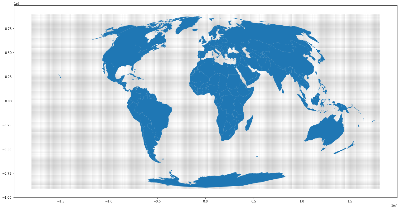
Preview Grid
base = grid.plot(figsize=(22,28), color='white', edgecolor='black', linewidth=0.1)
# combine with world geometry
plot = world.plot(ax=base)
Prepare binary search
The aggregation speed is important here and we should not use polygon intersection. Since we're working with a regular grid and floating point numbers, a binary search is likely one of the fastest ways for our context. numpy.digitize provides a binary search, but it must be adapted to for the spatial context. A lat or lng value is assigned to the nearest bin matching. We get our lat and lng bins from our original Mollweide grid, which are regularly spaced at 100km interval. Note that we need to do two binary searches, for lat and for lng values.
Create test points
testpoint = Point(8.546377, 47.392323)
testpoint2 = Point(13.726359, 51.028512)
gdf_testpoints = gp.GeoSeries([testpoint, testpoint2], crs=crs_wgs)
# project geometries to Mollweide
gdf_testpoints_proj = gdf_testpoints.to_crs(crs_proj)
gdf_testpoints_proj[0].x
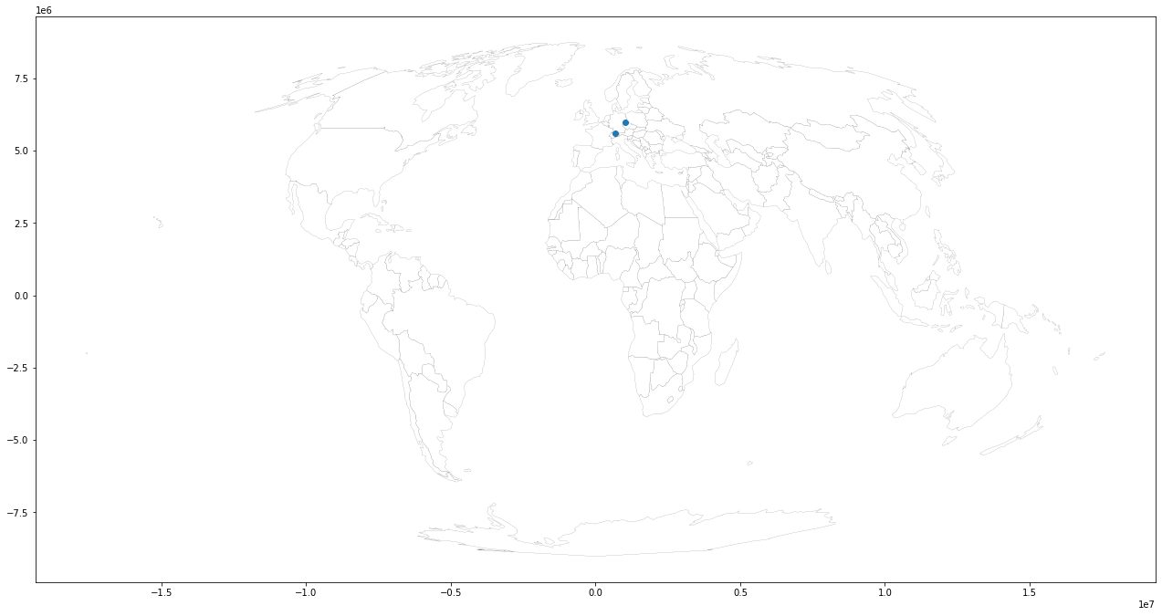
Preview map for testpoint
base = world.plot(figsize=(22,28), color='white', edgecolor='black', linewidth=0.1)
plot = gdf_testpoints_proj.plot(ax=base)
Use np.digitize() to assign coordinates to the grid
np.digitize is implemented in terms of np.searchsorted. This means that a binary search is used to bin the values, which scales much better for larger number of bins than the previous linear search. It also removes the requirement for the input array to be 1-dimensional.
Create 2 bins for each axis of existing Mollweide rows/cols grid:
ybins = np.array(rows)
xbins = np.array(cols)
Create 2 lists with a single entry (testpoint coordinate)
test_point_list_x = np.array([gdf_testpoints_proj[0].x, gdf_testpoints_proj[1].x])
test_point_list_y = np.array([gdf_testpoints_proj[0].y, gdf_testpoints_proj[1].y])
Find the nearest bin for x coordinate (returns the bin-index):
x_bin = np.digitize(test_point_list_x, xbins) - 1
display(x_bin)
Check value of bin (the y coordinate) based on returned index:
testpoint_xbin_idx = xbins[[x_bin[0], x_bin[1]]]
display(testpoint_xbin_idx)
Repeat the same for y-testpoint:
y_bin = np.digitize(test_point_list_y, ybins) - 1
display(y_bin)
testpoint_ybin_idx = ybins[[y_bin[0], y_bin[1]]]
display(testpoint_ybin_idx)
➡️ 759904 / 5579952 and 1059904 / 5979952 are indexes that we can use in our geodataframe index to return the matching grid-poly for each point
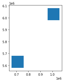
Highlight Testpoint in Grid
Get grid-poly by index from testpoint
grid.loc[testpoint_xbin_idx[0], testpoint_ybin_idx[0]]
Convert shapely bin poly to Geoseries and plot
testpoint_grids = gp.GeoSeries([grid.loc[testpoint_xbin_idx[0], testpoint_ybin_idx[0]].geometry, grid.loc[testpoint_xbin_idx[1], testpoint_ybin_idx[1]].geometry])
testpoint_grids.plot()
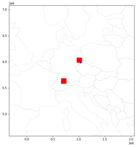
Preview map with testpoint and assigned bin
Set auto zoom with buffer:
minx, miny, maxx, maxy = testpoint_grids.total_bounds
buf = 1000000
# a figure with a 1x1 grid of Axes
fig, ax = plt.subplots(1, 1,figsize=(10,8))
ax.set_xlim(minx-buf, maxx+buf)
ax.set_ylim(miny-buf, maxy+buf)
base = world.plot(ax=ax, color='white', edgecolor='black', linewidth=0.1)
grid_base = testpoint_grids.plot(ax=base, facecolor='red', linewidth=0.1)
plot = gdf_testpoints_proj.plot(ax=grid_base, markersize=8, color='blue')
Prepare functions
Now that it has been visually verified that the algorithm works, lets create functions for the main processing job.
def get_best_bins(
    search_values_x: np.array, search_values_y: np.array,
    xbins: np.array, ybins: np.array) -> Tuple[np.ndarray, np.ndarray]:
    """Will return best bin for a lat and lng input

    Note: prepare bins and values in correct matching projection

    Args:
        search_values_y: A list of projected latitude values
        search_values_x: A list of projected longitude values
        xbins: 1-d array of bins to snap lat/lng values
        ybins: 1-d array of bins to snap lat/lng values

    Returns:
        Tuple[int, int]: A list of tuples with 2 index positions for the best
            matching bins for each lat/lng
    """
    xbins_idx = np.digitize(search_values_x, xbins, right=False)
    ybins_idx = np.digitize(search_values_y, ybins, right=False)
    return (xbins[xbins_idx-1], ybins[ybins_idx-1])
Test with LBSN data
We're going to test the binning of coordinates on a part of the YFCC geotagged images.
Prepare lat/lng tuple of lower left corner and upper right corner to crop sample map:
# Part of Italy and Sicily
bbox_italy = (
    7.8662109375, 36.24427318493909,
    19.31396484375, 43.29320031385282)
bbox = bbox_italy
Calculate bounding box with 1000 km buffer. For that, project the bounding Box to Mollweide, apply the buffer, and project back to WGS1984:
#convert to Mollweide
minx, miny = proj_transformer.transform(
    bbox_italy[0], bbox_italy[1])
maxx, maxy = proj_transformer.transform(
    bbox_italy[2], bbox_italy[3])
# apply buffer and convetr back to WGS1984
min_buf = proj_transformer_back.transform(minx-buf, miny-buf)
max_buf = proj_transformer_back.transform(maxx+buf, maxy+buf)
bbox_italy_buf = (min_buf[0], min_buf[1], max_buf[0], max_buf[1])
Select columns and types for improving speed
usecols = ['latitude', 'longitude']
dtypes = {'latitude': float, 'longitude': float}
reset_metrics(grid, metrics)
Load data
%%time
df = pd.read_csv(
    "yfcc_posts.csv", usecols=usecols, dtype=dtypes, encoding='utf-8')
print(len(df))
Filter on bounding box (Italy)
def filter_df_bbox(
    df: pd.DataFrame, bbox: Tuple[float, float, float, float],
    inplace: bool = True):
    """Filter dataframe with bbox on latitude and longitude column"""
    df.query(
        f'({bbox_italy_buf[0]} < longitude) & '
        f'(longitude <  {bbox_italy_buf[2]}) & '
        f'({bbox_italy_buf[1]} < latitude) & '
        f'(latitude < {bbox_italy_buf[3]})',
        inplace=True)
    # set index to asc integers
    if inplace:
        df.reset_index(inplace=True, drop=True)
        return
    return df.reset_index(inplace=False, drop=True)
Execute and count number of posts in the bounding box:
%%time
filter_df_bbox(df=df, bbox=bbox_italy_buf)
print(f"There're {len(df):,.0f} YFCC geotagged posts located within the bounding box.")
df.head()
Project coordinates to Mollweide
Projection speed can be increased by using a predefined pyproj.Transformer. We're also splitting our input-dataframe into a list of dataframe, each containing 1 Million records, so we can process the data in chunks.
def proj_df(df, proj_transformer):
    """Project pandas dataframe latitude and longitude decimal degrees
    using predefined proj_transformer"""
    if 'longitude' not in df.columns:
        return
    xx, yy = proj_transformer.transform(
        df['longitude'].values, df['latitude'].values)
    # assign projected coordinates to
    # new columns x and y
    # the ':' means: replace all values in-place
    df.loc[:, "x"] = xx
    df.loc[:, "y"] = yy
    # Drop WGS coordinates
    df.drop(columns=['longitude', 'latitude'], inplace=True)
%%time
proj_df(df, proj_transformer)
print(f'Projected {len(df.values):,.0f} coordinates')
df.head()
Perform the bin assignment
%%time
xbins_match, ybins_match = get_best_bins(
    search_values_x=df['x'].to_numpy(),
    search_values_y=df['y'].to_numpy(),
    xbins=xbins, ybins=ybins)
len(xbins_match)
xbins_match[:10]
ybins_match[:10]
A: Post Count per grid
Attach target bins to original dataframe. The : means: modify all values in-place
df.loc[:, 'xbins_match'] = xbins_match
df.loc[:, 'ybins_match'] = ybins_match
# set new index column
df.set_index(['xbins_match', 'ybins_match'], inplace=True)
# drop x and y columns not needed anymore
df.drop(columns=['x', 'y'], inplace=True)
df.head()
Count per bin:
%%time
cardinality_series = df.groupby(
        df.index).size()
cardinality_series.index = pd.MultiIndex.from_tuples(
        cardinality_series.index, names=['xbin', 'ybin'])
cardinality_series.head()
reset_metrics(grid, ["postcount"], setzero=True)
Append Series with calculated counts to grid (as new column) based on index match:
grid.loc[cardinality_series.index, 'postcount'] = cardinality_series
grid[grid["postcount"] > 0].head()
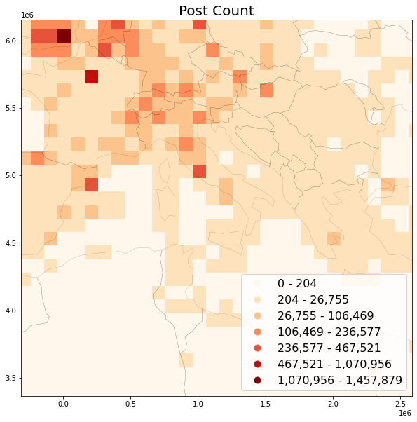
Preview post count map
# create bounds from WGS1984 italy and project to Mollweide
minx, miny = proj_transformer.transform(
    bbox_italy[0], bbox_italy[1])
maxx, maxy = proj_transformer.transform(
    bbox_italy[2], bbox_italy[3])
Use headtail_breaks classification scheme because it is specifically suited to map long tailed data, see Jiang 2013
- Jiang, B. (August 01, 2013). Head/Tail Breaks: A New Classification Scheme for Data with a Heavy-Tailed Distribution. The Professional Geographer, 65, 3, 482-494.
# global legend font size setting
plt.rc('legend', **{'fontsize': 16})

def leg_format(leg):
    "Format matplotlib legend entries"
    for lbl in leg.get_texts():
        label_text = lbl.get_text()
        lower = label_text.split()[0]
        upper = label_text.split()[2]
        new_text = f'{float(lower):,.0f} - {float(upper):,.0f}'
        lbl.set_text(new_text)

def title_savefig_mod(title, save_fig):
    """Update title/output name if grid size is not 100km"""
    if GRID_SIZE_METERS == 100000:
        return title, save_fig
    km_size = GRID_SIZE_METERS/1000
    title = f'{title} ({km_size:.0f}km grid)'
    if save_fig:
        save_fig = save_fig.replace(
            '.png', f'_{km_size:.0f}km.png')
    return title, save_fig

def save_plot(
    grid: gp.GeoDataFrame, title: str, column: str, save_fig: str = None):
    """Plot GeoDataFrame with matplotlib backend, optionaly export as png"""
    fig, ax = plt.subplots(1, 1,figsize=(10,12))
    ax.set_xlim(minx-buf, maxx+buf)
    ax.set_ylim(miny-buf, maxy+buf)
    title, save_fig = title_savefig_mod(
        title, save_fig)
    ax.set_title(title, fontsize=20)
    base = grid.plot(
        ax=ax, column=column, cmap='OrRd', scheme='headtail_breaks',
        legend=True, legend_kwds={'loc': 'lower right'})
    # combine with world geometry
    plot = world.plot(
        ax=base, color='none', edgecolor='black', linewidth=0.1)
    leg = ax.get_legend()
    leg_format(leg)
    if not save_fig:
        return
    fig.savefig(Path("OUT") / save_fig, dpi=300, format='PNG',
                bbox_inches='tight', pad_inches=1)
save_plot(
    grid=grid, title='Post Count',
    column='postcount', save_fig='postcount_sample.png')
B: User Count per grid
When using RAW data, the caveat for calculating usercounts is that all distinct ids per bin must be present first, before calculating the total count. Since the input data (Social Media posts) is spatially unordered, this requires either a two-pass approach (e.g. writing intermediate data to disk and performing the count in a second pass), or storing all user guids per bin in-memory. We're using the second approach here.
What can be done to reduce memory load is to process the input data in chunks. After each chunk has been processed, Python's garbage collection can do its work and remove everything that is not needed anymore.
Furthermore, we can store intermediate data to CSV, which is also more efficient than loading data from DB.
These ideas are combined in the methods below. Adjust default chunk_size of 5000000 to your needs.
Specify input data
First, specify the columns that need to be retrieved from the database. In addition to lat and lng, we need the user_guid for calculating usercounts.
usecols = ['latitude', 'longitude', 'user_guid']
Adjust method for stream-reading from CSV in chunks:
%%time
chunk_size = 5000000
iter_csv = pd.read_csv(
    "yfcc_posts.csv", usecols=usecols, iterator=True,
    dtype=dtypes, encoding='utf-8', chunksize=chunk_size)
def proj_report(df, proj_transformer, cnt, inplace: bool = False):
    """Project df with progress report"""
    proj_df(df, proj_transformer)
    clear_output(wait=True)
    print(f'Projected {cnt:,.0f} coordinates')
    if inplace:
        return
    return df
%%time
# filter
chunked_df = [
    filter_df_bbox(
        df=chunk_df, bbox=bbox_italy_buf, inplace=False)
    for chunk_df in iter_csv]

# project
projected_cnt = 0
for chunk_df in chunked_df:
    projected_cnt += len(chunk_df)
    proj_report(
        chunk_df, proj_transformer, projected_cnt, inplace=True)

chunked_df[0].head()
Perform the bin assignment and count distinct users
First assign coordinates to bin using our binary search:
def bin_coordinates(
        df: pd.DataFrame, xbins:
        np.ndarray, ybins: np.ndarray) -> pd.DataFrame:
    """Bin coordinates using binary search and append to df as new index"""
    xbins_match, ybins_match = get_best_bins(
        search_values_x=df['x'].to_numpy(),
        search_values_y=df['y'].to_numpy(),
        xbins=xbins, ybins=ybins)
    # append target bins to original dataframe
    # use .loc to avoid chained indexing
    df.loc[:, 'xbins_match'] = xbins_match
    df.loc[:, 'ybins_match'] = ybins_match
    # drop x and y columns not needed anymore
    df.drop(columns=['x', 'y'], inplace=True)
def bin_chunked_coordinates(
    chunked_df: List[pd.DataFrame]):
    """Bin coordinates of chunked dataframe"""
    binned_cnt = 0
    for ix, df in enumerate(chunked_df):
        bin_coordinates(df, xbins, ybins)
        df.set_index(['xbins_match', 'ybins_match'], inplace=True)
        clear_output(wait=True)
        binned_cnt += len(df)
        print(f"Binned {binned_cnt:,.0f} coordinates..")
%%time
bin_chunked_coordinates(chunked_df)
chunked_df[0].head()
Now group user_guids per bin in distinct sets. The demonstration below is based the first chunk of posts ([0]):
%%time
df = chunked_df[0]
series_grouped = df["user_guid"].groupby(
        df.index).apply(set)
series_grouped.head()
Now we have sets of user_guids per bin. The next step is to count the number of distinct items in each set:
%%time
cardinality_series = series_grouped.apply(len)
cardinality_series.head()
To be able to process all user_guids in chunks, we need to union sets incrementally and, finally, attach distinct user count to grid, based on composite index (bin-ids). This last part of the process is the same as in counting posts.
def init_col_emptysets(
    df: Union[pd.DataFrame, gp.GeoDataFrame], col_name: str):
    """Initialize column of dataframe with empty sets."""
    grid[col_name] = [set() for x in range(len(grid.index))]
def union_sets_series(
    set_series: pd.Series, set_series_other: pd.Series) -> pd.Series:
    """Union of two pd.Series of sets based on index, with keep set index"""
    return pd.Series(
        [set.union(*z) for z in zip(set_series, set_series_other)],
        index=set_series.index)

def group_union_chunked(
    chunked_df: List[pd.DataFrame], grid: gp.GeoDataFrame,
    col: str = "user_guid", metric: str = "usercount"):
    """Group dataframe records per bin, create distinct sets,
    calculate cardinality and append to grid"""
    # init grid empty sets
    init_col_emptysets(grid, f"{metric}_set")
    for ix, df in enumerate(chunked_df):
        series_grouped = df[col].groupby(
            df.index).apply(set)
        # series of new user_guids per bin
        series_grouped.index = pd.MultiIndex.from_tuples(
            series_grouped.index, names=['xbin', 'ybin'])
        # series of existing user_guids per bin
        existing_sets_series = grid.loc[
            series_grouped.index, f"{metric}_set"]
        # union existing & new
        series_grouped = union_sets_series(
            series_grouped, existing_sets_series)
        grid.loc[series_grouped.index, f'{metric}_set'] = series_grouped
        clear_output(wait=True)
        print(f"Grouped {(ix*chunk_size)+len(df):,.0f} {col}s..")

    # after all user_guids have been processed to bins,
    # calculate cardinality and drop user_guids to free up memory
    grid[metric] = grid[f'{metric}_set'].apply(len)
    grid.drop(columns=[f'{metric}_set'], inplace=True)
%%time
group_union_chunked(
    chunked_df=chunked_df, grid=grid,
    col="user_guid", metric="usercount")
grid[grid["usercount"]> 0].head()
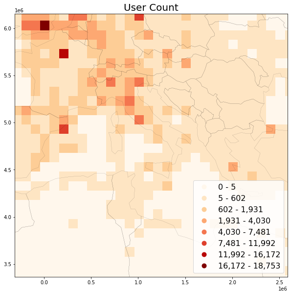
Preview user count map
save_plot(
    grid=grid, title='User Count',
    column='usercount', save_fig='usercount_sample.png')
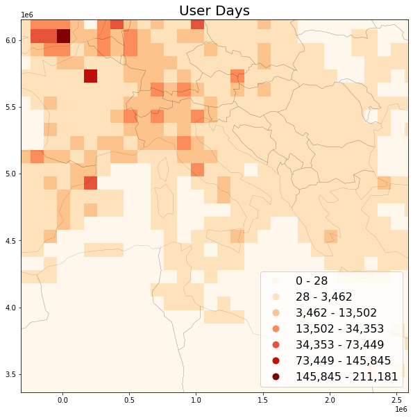
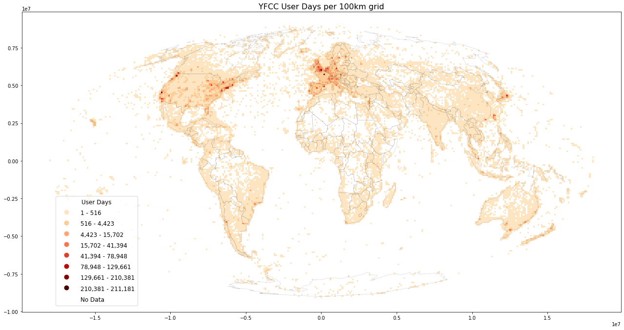
C: User Days
Wood, Guerry, Silver and Lacayo (2013) found that frequency of Flickr users per month correlates with official visitation rates for National Parks in the USA and further coined the term “user days” as a measurement for “the total number of days, across all users, that each person took at least one photograph within each site” (ibid, p. 6). User days has emerged as a suitable intermediate metric, between post count and user count.
To calculate user days, we need to query additional YFCC post attribute post_create_date. This requiress overriding get_col_ref() method:
usecols = ['latitude', 'longitude', 'user_guid', 'post_create_date']
Get data from CSV (define a method this time):
def read_project_chunked(filename: str,
    usecols: List[str], chunk_size: int =5000000,
    bbox: Tuple[float, float, float, float] = None) -> List[pd.DataFrame]:
    """Read data from csv, optionally clip to bbox and projet"""
    iter_csv = pd.read_csv(
        filename, usecols=usecols, iterator=True,
        dtype=dtypes, encoding='utf-8', chunksize=chunk_size)
    if bbox:
        chunked_df = [filter_df_bbox(
            df=chunk_df, bbox=bbox, inplace=False)
        for chunk_df in iter_csv]
    else:
        chunked_df = [chunk_df for chunk_df in iter_csv]
    # project
    projected_cnt = 0
    for chunk_df in chunked_df:
        projected_cnt += len(chunk_df)
        proj_report(
            chunk_df, proj_transformer, projected_cnt, inplace=True)
    return chunked_df
Run:
%%time
chunked_df = read_project_chunked(
    filename="yfcc_posts.csv",
    usecols=usecols,
    bbox=bbox_italy_buf)
chunked_df[0].head()
%%time
bin_chunked_coordinates(chunked_df)
chunked_df[0].head()
To count distinct userdays, concat user_guid and post_create_date into single column:
%%time
def concat_cols_df(
    df: pd.DataFrame, col1: str, col2: str, col_out: str):
    """Concat dataframe values of col1 and col2 into new col"""
    df[col_out] = df[col1] + df[col2]
    df.drop(columns=[col1, col2], inplace=True)
%%time
for df in chunked_df:
    concat_cols_df(
        df, col1="user_guid",
        col2="post_create_date",
        col_out="user_day")
chunked_df[0].head()
Count distinct userdays and attach counts to grid. The process is now the same as in counting distinct users:
%%time
group_union_chunked(
    chunked_df=chunked_df, grid=grid,
    col="user_day", metric="userdays")
grid[grid["userdays"]> 0].head()
save_plot(
    grid=grid, title='User Days',
    column='userdays', save_fig='userdays_sample.png')
There're other approaches for further reducing noise. For example, to reduce the impact of automatic capturing devices (such as webcams uploading x pictures per day), a possibility is to count distinct userlocations. For userlocations metric, a user would be counted multiple times per grid bin only for pictures with different lat/lng. Or the number of distinct userlocationdays (etc.). These metrics are easy to implement using hll, but quite difficult to compute using raw data.
Prepare methods
Lets summarize the above code in a few methods:
def group_count(
    df: pd.DataFrame) -> pd.Series:
    """Group dataframe by composite index and return count of duplicate indexes

        Args:
        df: Indexed dataframe (with duplicate indexes).
    """
    series_grouped = df.groupby(
            df.index).size()
    # split tuple index to produce
    # the multiindex of the original dataframe
    # with xbin and ybin column names
    series_grouped.index = pd.MultiIndex.from_tuples(
        series_grouped.index, names=['xbin', 'ybin'])
    # return column as indexed pd.Series
    return series_grouped
Plotting preparation
The below methods contain combined code from above, plus final plot style improvements.
def format_legend(
    leg, bounds: List[str], inverse: bool = None,
    metric: str = "postcount"):
    """Formats legend (numbers rounded, colors etc.)"""
    leg.set_bbox_to_anchor((0., 0.2, 0.2, 0.2))
    # get all the legend labels
    legend_labels = leg.get_texts()
    plt.setp(legend_labels, fontsize='12')
    lcolor = 'black'
    if inverse:
        frame = leg.get_frame()
        frame.set_facecolor('black')
        frame.set_edgecolor('grey')
        lcolor = "white"
    plt.setp(legend_labels, color = lcolor)
    if metric == "postcount":
        leg.set_title("Post Count")
    elif metric == "usercount":
        leg.set_title("User Count")
    else:
        leg.set_title("User Days")
    plt.setp(leg.get_title(), fontsize='12')
    leg.get_title().set_color(lcolor)
    # replace the numerical legend labels
    for bound, legend_label in zip(bounds, legend_labels):
        legend_label.set_text(bound)
def format_bound(
    upper_bound: float = None, lower_bound: float = None) -> str:
    """Format legend text for class bounds"""
    if upper_bound is None:
        return f'{lower_bound:,.0f}'
    if lower_bound is None:
        return f'{upper_bound:,.0f}'
    return f'{lower_bound:,.0f} - {upper_bound:,.0f}'

def get_label_bounds(
    scheme_classes, metric_series: pd.Series,
    flat: bool = None) -> List[str]:
    """Get all upper bounds in the scheme_classes category"""
    upper_bounds = scheme_classes.bins
    # get and format all bounds
    bounds = []
    for idx, upper_bound in enumerate(upper_bounds):
        if idx == 0:
            lower_bound = metric_series.min()
        else:
            lower_bound = upper_bounds[idx-1]
        if flat:
            bound = format_bound(
                lower_bound=lower_bound)
        else:
            bound = format_bound(
                upper_bound, lower_bound)
        bounds.append(bound)
    if flat:
        upper_bound = format_bound(
            upper_bound=upper_bounds[-1])
        bounds.append(upper_bound)
    return bounds

def label_nodata(
    grid: gp.GeoDataFrame, inverse: bool = None,
    metric: str = "postcount"):
    """Add white to a colormap to represent missing value

    Adapted from:
        https://stackoverflow.com/a/58160985/4556479

    See available colormaps:
        http://holoviews.org/user_guide/Colormaps.html
    """
    # set 0 to NaN
    grid_nan = grid[metric].replace(0, np.nan)
    # get headtail_breaks
    # excluding NaN values
    headtail_breaks = mc.HeadTailBreaks(
        grid_nan.dropna())
    grid[f'{metric}_cat'] = headtail_breaks.find_bin(
        grid_nan).astype('str')
    # set label for NaN values
    grid.loc[grid_nan.isnull(), f'{metric}_cat'] = 'No Data'
    bounds = get_label_bounds(
        headtail_breaks, grid_nan.dropna().values)
    cmap_name = 'OrRd'
    nodata_color = 'white'
    if inverse:
        nodata_color = 'black'
        cmap_name = 'fire'
    cmap = plt.cm.get_cmap(cmap_name, headtail_breaks.k)
    # get hex values
    cmap_list = [colors.rgb2hex(cmap(i)) for i in range(cmap.N)]
    # lighten or darken up first/last color a bit
    # to offset from black or white background
    if inverse:
        firstcolor = '#3E0100'
        cmap_list[0] = firstcolor
    else:
        lastcolor = '#440402'
        cmap_list.append(lastcolor)
        cmap_list.pop(0)
    # append nodata color
    cmap_list.append(nodata_color)
    cmap_with_nodata = colors.ListedColormap(cmap_list)
    return cmap_with_nodata, bounds

def plot_figure(
    grid: gp.GeoDataFrame, title: str, inverse: bool = None,
    metric: str = "postcount", store_fig: str = None):
    """Combine layers and plot"""
    # for plotting, there're some minor changes applied
    # to the dataframe (replace NaN values),
    # make a shallow copy here to prevent changes
    # to modify the original grid
    grid_plot = grid.copy()
    # create new plot figure object with one axis
    fig, ax = plt.subplots(1, 1, figsize=(22,28))
    ax.set_title(title, fontsize=16)
    print("Classifying bins..")
    cmap_with_nodata, bounds = label_nodata(
        grid=grid_plot, inverse=inverse, metric=metric)
    base = grid_plot.plot(
        ax=ax,
        column=f'{metric}_cat', cmap=cmap_with_nodata, legend=True)
    leg = ax.get_legend()
    print("Formatting legend..")
    format_legend(leg, bounds, inverse, metric)
    # combine with world geometry
    edgecolor = 'black'
    if inverse:
        edgecolor = 'white'
    clear_output(wait=True)
    plot = world.plot(
        ax=base, color='none', edgecolor=edgecolor, linewidth=0.1)
    if store_fig:
        print("Storing figure as png..")
        if inverse:
            store_fig = store_fig.replace('.png', '_inverse.png')
        plot.get_figure().savefig(
            Path("OUT") / store_fig, dpi=300, format='PNG',
            bbox_inches='tight', pad_inches=1)
def filter_nullisland_df(
    df: pd.DataFrame, col_x: str = "longitude", col_y: str = "latitude"):
    """Remove records from df inplace where both x and y coordinate are 0"""
    if col_x in df.columns:
        df.query(
            f'({col_x} == 0 and {col_y} == 0) == False', inplace=True)

def load_plot(
    filename: str, grid: gp.GeoDataFrame, title: str, inverse: bool = None,
    metric: str = "postcount", store_fig: str = None, store_pickle: str = None,
    chunk_size: int = 5000000):
    """Load data, bin coordinates, estimate distinct counts (cardinality) and plot map

        Args:
        filename: Filename to read and write intermediate data
        grid: A geopandas geodataframe with indexes x and y
            (projected coordinates) and grid polys
        title: Title of the plot
        inverse: If True, inverse colors (black instead of white map)
        metric: target column for aggregate. Default: postcount_est.
        store_fig: Provide a name to store figure as PNG. Will append
            '_inverse.png' if inverse=True.
        store_pickle: Provide a name to store pickled dataframe
            with aggregate counts to disk
        chunk_size: chunk processing into x records per chunk
    """
    usecols = ['latitude', 'longitude']
    if metric != "postcount":
        usecols.append('user_guid')
    if metric == "userdays":
        usecols.append('post_create_date')
    # get data from CSV
    chunked_df = read_project_chunked(
        filename=filename,
        usecols=usecols)
    # bin coordinates
    bin_chunked_coordinates(chunked_df)
    # reset metric column
    reset_metrics(grid, [metric], setzero=True)
    print("Getting cardinality per bin..")
    if metric == "postcount":
        cardinality_cnt = 0
        for df in chunked_df:
            cardinality_series = group_count(
                df)
            # update postcounts per grid-bin based on index,
            # use += to allow incremental update
            grid.loc[
                cardinality_series.index,
                'postcount'] += cardinality_series
            cardinality_cnt += len(df)
            clear_output(wait=True)
            print(f"{cardinality_cnt:,.0f} posts processed.")
    else:
        col = "user_guid"
        if metric == "userdays":
            # concat user_guid and
            # post_create_date
            for df in chunked_df:
                concat_cols_df(
                    df, col1="user_guid",
                    col2="post_create_date",
                    col_out="user_day")
            col = "user_day"
        group_union_chunked(
            chunked_df=chunked_df, grid=grid,
            col=col, metric=metric)
    print("Storing aggregate data as pickle..")
    if store_pickle:
        grid.to_pickle(Path("OUT") / store_pickle)
    print("Plotting figure..")
    plot_figure(grid, title, inverse, metric, store_fig)
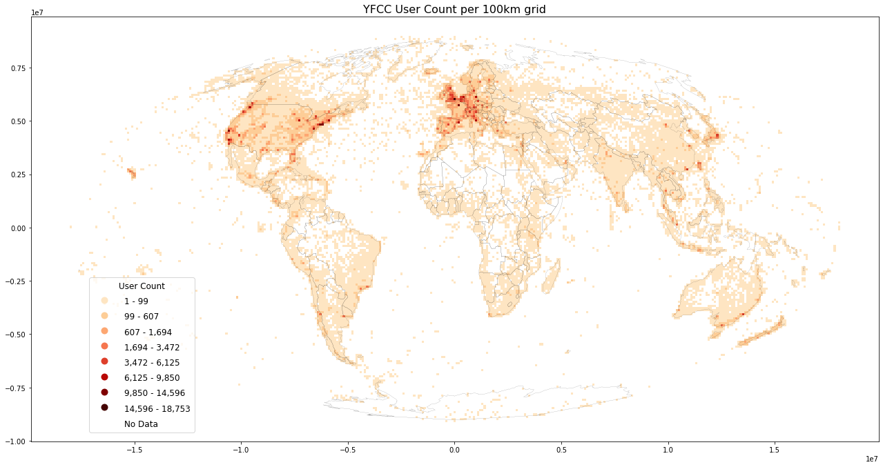
Plotting worldmaps: Post Count, User Count and User Days
Plot worldmap for each datasource
reset_metrics(grid, ["postcount", "usercount", "userdays"])
%%time
%%memit
load_plot(
    grid=grid, filename='yfcc_posts.csv', title=f'YFCC Post Count per {int(length/1000)}km grid',
    inverse=False, store_fig="yfcc_postcount.png")

%%time
%%memit
load_plot(
    grid=grid, filename='yfcc_posts.csv', title=f'YFCC User Count per {int(length/1000)}km grid',
    inverse=False, store_fig="yfcc_usercount.png",
    metric="usercount")
%%time
%%memit
load_plot(
    grid=grid, filename='yfcc_posts.csv', title=f'YFCC User Days per {int(length/1000)}km grid',
    inverse=False, store_fig="yfcc_userdays.png",
    metric="userdays")
Have a look at the final grid with cardinality (distinct counts) for postcount, usercount and userdays
An immediate validation is to verify that postcount >= userdays >= usercount.
grid[grid["postcount"]>1].head()
Store results to CSV for archive purposes:
Define method
def grid_agg_tocsv(
    grid: gp.GeoDataFrame, filename: str,
    metrics: List[str] = ["postcount", "usercount", "userdays"]):
    """Store geodataframe aggregate columns and indexes to CSV"""
    grid.to_csv(filename, mode='w', columns=metrics, index=True)
Convert/store to CSV (aggregate columns and indexes only):
grid_agg_tocsv(grid, "yfcc_all_raw.csv")
def create_new_grid(length: int = 100000, width: int = 100000) -> gp.GeoDataFrame:
    """Create new 100x100km grid GeoDataFrame (Mollweide)"""
    # Mollweide projection epsg code
    epsg_code = 54009
    crs_proj = f"esri:{epsg_code}"
    crs_wgs = "epsg:4326"
    # define Transformer ahead of time
    # with xy-order of coordinates
    proj_transformer = Transformer.from_crs(
        crs_wgs, crs_proj, always_xy=True)
    # grid bounds from WGS1984 to Mollweide
    xmin = proj_transformer.transform(
        -180, 0)[0]
    xmax = proj_transformer.transform(
        180, 0)[0]
    ymax = proj_transformer.transform(
        0, 90)[1]
    ymin = proj_transformer.transform(
        0, -90)[1]
    # define grid size
    length = length
    width = width
    grid = create_grid_df(
        length=length, width=width,
        xmin=xmin, ymin=ymin,
        xmax=xmax, ymax=ymax)
    # convert grid DataFrame to grid GeoDataFrame
    grid = grid_to_gdf(grid)
    return grid

def grid_agg_fromcsv(
    filename: str, metrics: List[str] = ["postcount", "usercount", "userdays"],
    length: int = 100000, width: int = 100000):
    """Create a new Mollweide grid GeoDataFrame and
    attach aggregate data columns from CSV based on index"""
    # 1. Create new 100x100km (e.g.) grid
    grid = create_new_grid(length=length, width=width)
    # 2. load aggregate data from CSV and attach to grid
    # -----
    types_dict = dict()
    for metric in metrics:
        types_dict[metric] = int
    df = pd.read_csv(
        filename, dtype=types_dict, index_col=["xbin", "ybin"])
    # join columns based on index
    grid = grid.join(df)
    # return grid with aggregate data attached
    return grid
To create a new grid and load aggregate counts from CSV:
grid = grid_agg_fromcsv(
    "yfcc_all.csv", length=length, width=width)
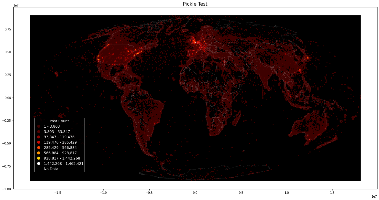
Load & plot pickled dataframe
Loading (geodataframe) using pickle. This is the easiest way to store intermediate data, but may be incompatible if package versions change. If loading pickles does not work, a workaround is to load data from CSV and re-create pickle data, which will be compatible with used versions.
Store results using pickle for later resuse:
grid.to_pickle("yfcc_all_raw.pkl")
Load pickled dataframe:
%%time
grid = pd.read_pickle("yfcc_all_raw.pkl")
Then use plot_figure on dataframe to plot with new parameters, e.g. plot inverse:
plot_figure(grid, "Pickle Test", inverse=True, metric="postcount")
Interactive Map with Holoviews/ Geoviews
In the hll notebook, we'll combine raw and hll results in an interactive map. Follow in 03_yfcc_gridagg_hll.ipynb