Introduction
Based on data from YFCC100m dataset, this Notebook introduces basics and usage of the privacy-aware data structure. The data used here was converted from the raw lbsn structure to its privacy-aware version, which is based, at its core, on the HyperLogLog (HLL) algorithm.
The raw lbsn structure was developed to systematically characterize LBSN data aspects in a common scheme that enables privacy-by-design for connected software, data handling and information visualization. The components of the raw structure are documented here.
The hll structure is more or less a convention for systematically converting raw structure components to a privacy-aware format that is based on HLL. A possible data scheme is proposed here. It is critical to note that not all components of the privacy-aware structure need to be available for all visualizations. Rather, an analyst will need to consider, on a per visualization basis, which components are needed. Therefore, the proposed structure is not exhaustive and should be treated as a demonstrator that can be extended.
In this Notebook, we introduce the basic process of working with the privacy-aware hll structure. This is the first notebook in a tutorial series of three notebooks:
- 1) the HLL Introduction (01_hll_intro.ipynb) explaines basic concepts and tools for working with the privacy-aware lbsn data
- 2) the RAW Notebook (02_yfcc_gridagg_raw.ipynb) demonstrates how a typical grid-based visualization looks like when using the raw lbsn structure and
- 3) the HLL Notebook (03_yfcc_gridagg_hll.ipynb) demonstrates the same visualization using the privacy-aware hll lbsn structure
Additional notes:
Use Shift+Enter to walk through the Notebook
Preparations
Load dependencies
import os
import psycopg2 # Postgres API
import geoviews as gv
import holoviews as hv
import pandas as pd
import numpy as np
import warnings
with warnings.catch_warnings():
    # prevent missing glyph warnings
    warnings.simplefilter("ignore")
    import matplotlib.pyplot as plt
from collections import namedtuple
from geoviews import opts
from holoviews import dim
from cartopy import crs as ccrs
from IPython.display import display, Markdown
# init bokeh
from modules import preparations
preparations.init_imports()
pd.set_option('display.max_colwidth', 25)


Define credentials as environment variables
db_user = "postgres"
db_pass = os.getenv('POSTGRES_PASSWORD')
# set connection variables
db_host = "hlldb"
db_port = "5432"
db_name = "hlldb"
Connect to empty Postgres database running HLL Extension. Note that only readonly privileges are needed.
db_connection = psycopg2.connect(
        host=db_host,
        port=db_port,
        dbname=db_name,
        user=db_user,
        password=db_pass
)
db_connection.set_session(readonly=True)
Test connection:
db_query = """
    SELECT 1;
"""
# create pandas DataFrame from database data
df = pd.read_sql_query(db_query, db_connection)
display(df.head())
from modules import tools
db_conn = tools.DbConn(db_connection)
db_conn.query("SELECT 1;")
Privacy-aware data introduction
The privacy-aware structure is based on two basic components, 1) the overlay and 2) the base. The overlay defines what is measured, which can be, for example, number of users (_userhll), number of posts (_posthll), or number of userdays (_datehll). Overlays are stored as HyperLogLog (HLL) sets, which contain statistically approximated versions of original data. It is possible to get an approximation of counts by calculating the cardinality of a HLL Set.
Conversely, the base is the context for which measurements are analyzed. The base can be terms, location-terms, dates, coordinates, places, or any combinations or complex queries. Herein, our base are lat-lng coordinates. Bases also have some privacy implications, particularly when they're accurate enough so that only one person is referenced (e.g. a latitude-longitude pair with high accuracy).
The core aim of the privacy-aware structure is to support visual analytics where no original data is needed. By removing the need for original data, entire process pipelines (such as Monitoring) can be converted to privacy-aware versions, without loosing quality or validity for interpretation.
For calculating with HLL Sets, it is necessary to connect to a Postgres Database which runs the Citus HLL extension. The database itself can be empty, it is only needed for calculation. A docker container for an empty postgres database with Citus HLL extension is made available here.
First, some statistics for the data we're working with.
%%time
db_query = """
    SELECT count(*) FROM spatial.latlng t1;
"""

display(Markdown(
    f"There're "
    f"<strong style='color: red;'>"
    f"{db_conn.query(db_query)['count'][0]:,.0f}</strong> "
    f"distinct coordinates in this table."))
The Flickt YFCC 100M dataset includes 99,206,564 photos and 793,436 videos from 581,099 different photographers, and 48,469,829 of those are geotagged [1].
In the privacy-aware HLL data we're working with, distinct users, posts and dates have been grouped
by various means such as distinct latitude/longitude pairs. The number of distinct coordinates can be calculated from
the table spatial.latlng.
db_query = tools.get_stats_query("spatial.latlng")
stats_df = db_conn.query(db_query)
stats_df["bytes/ct"] = stats_df["bytes/ct"].fillna(0).astype('int64')
display(stats_df)
Data structure preview (get random 10 records):
db_query = "SELECT * FROM spatial.latlng ORDER BY RANDOM() LIMIT 10;"
first_10_df = db_conn.query(db_query)
display(first_10_df)
Did you know that you can see the docstring from defined functions with ?? This helps us remember what functions are doing:
db_conn.query?
Test cardinality calculation: hll_add_agg() is used to create a HLL set consisting of 3 distinct sample ids, hll_cardinality() is then applied to retrieve the cardinality of the set (the number of distinct elements).
db_query = """
    SELECT hll_cardinality(hll_add_agg(hll_hash_text(a)))
    FROM (
    VALUES ('24399297324604'), ('238949132532500'), ('269965843254300')
    ) s(a);
"""
# create pandas DataFrame from database data
df = db_conn.query(db_query)
display(df.head())
Example Cardinality
Have a look at a random number of coordinates from our YFCC spatial.latlng table
HllRecord = namedtuple(
    'Hll_record', 'lat, lng, user_hll, post_hll, date_hll')

def strip_item(item, strip: bool):
    if not strip:
        return item
    if len(item) > 120:
        item = item[:120] + '..'
    return item


def get_hll_record(record, strip: bool = None):
    """Concatenate topic info from post columns"""

    lat = record.get('latitude')
    lng = record.get('longitude')
    user_hll = strip_item(record.get('user_hll'), strip)
    post_hll = strip_item(record.get('post_hll'), strip)
    date_hll = strip_item(record.get('date_hll'), strip)
    return HllRecord(lat, lng, user_hll, post_hll, date_hll)

hll_sample_records = []
for ix, hll_record in first_10_df.iterrows():
    hll_record = get_hll_record(hll_record)
    print(
        f'Coordinate: {hll_record.lat}, {hll_record.lng}, '
        f'Post Count (Hll-Set): {hll_record.post_hll}, '
        f'User Count (Hll-Set): {hll_record.user_hll}')
    hll_sample_records.append(hll_record)
Lets calculate the cardinality (the estimated count) of these sets:
db_query = f"""
SELECT hll_cardinality(user_hll)::int as usercount
FROM (VALUES
          ('{hll_sample_records[0].user_hll}'::hll),
          ('{hll_sample_records[1].user_hll}'::hll),
          ('{hll_sample_records[2].user_hll}'::hll),
          ('{hll_sample_records[3].user_hll}'::hll),
          ('{hll_sample_records[4].user_hll}'::hll),
          ('{hll_sample_records[5].user_hll}'::hll),
          ('{hll_sample_records[6].user_hll}'::hll),
          ('{hll_sample_records[7].user_hll}'::hll),
          ('{hll_sample_records[8].user_hll}'::hll),
          ('{hll_sample_records[9].user_hll}'::hll)
        ) s(user_hll)
ORDER BY usercount DESC;
"""

df = db_conn.query(db_query)
# combine with base data
df["lat"] = [record.lat for record in hll_sample_records]
df["lng"] = [record.lng for record in hll_sample_records]
df.set_index(['lat', 'lng'])
Lets take this apart:
- the
f''format refers to f-strings python format, where variables can be substituted with curly brackets, e.g.{hll_sample_records[0].user_hll}, which inserts a HLL-Set as a string from our CSV - by surrounding the HLL-Set with single-quotes, e.g.
'HLL-Set', it is treated as a string in SQL - adding
::hllafter the string labels the record as the special typehll. This is called type casting, and it doesn't change the content of the value hll_cardinality(user_hll)::intmeans, for eachuser_hll, calculate the cardinality (the approximated count of distinct values in the set- since this aproximation is a float, we cast it to an int using
::int
The result shows that all coordinates were only frequented by 1 user from the YFCC dataset.
Calculating with HLL Sets
What is interesting here: HLL-Sets can be combined or intersected. E.g.:
db_query = f"""
SELECT hll_cardinality(hll_union_agg(s.a))::int
FROM (
    VALUES ('{hll_sample_records[1].user_hll}'::hll),
           ('{hll_sample_records[2].user_hll}'::hll)
) s(a)
"""
df = db_conn.query(db_query)
df.head()
Obviously, the users who frequented the two coordinates were different.
HLL Modes
The postgres implementation of citus has several modes, for reasons of performance:
A hll is a combination of different set/distinct-value-counting algorithms that can be thought of as a hierarchy, along with rules for moving up that hierarchy. In order to distinguish between said algorithms, we have given them names:
EMPTY A constant value that denotes the empty set.
EXPLICIT An explicit, unique, sorted list of integers in the set, which is maintained up to a fixed cardinality.
SPARSE A 'lazy', map-based implementation of HyperLogLog, a probabilistic set data structure. Only stores the indices and values of non-zero registers in a map, until the number of non-zero registers exceeds a fixed cardinality.
FULL A fully-materialized, list-based implementation of HyperLogLog. Explicitly stores the value of every register in a list ordered by register index.
If used in a privacy-aware context, explicit mode does not provide any improvement, since unique ids are store fully, which can be reversed. Sparse mode, according to Desfontaines, Lochbihler, & Basin (2018), may be more vulnerable to reverse engeneering attacks since it provides more accurate information on each mapped unique id.
It is possible to tune the hll mode with SELECT hll_set_defaults(log2m, regwidth, expthresh, sparseon); The default values are:
DEFAULT_LOG2M 11DEFAULT_REGWIDTH 5DEFAULT_EXPTHRESH -1- explicit mode onDEFAULT_SPARSEON 1- auto sparse mode
Disable the explicit mode with the following command for the current connection (Note: the output will return the settings before the change):
df = db_conn.query("SELECT hll_set_defaults(11,5, 0, 1);")
df.head()
It is also possible to define the exact number of ids in a hll set, when the promotion to a full hll set occurs. By default (-1), this is automatically determined based on storage efficiency. Our observation was that promotion to full mode typically occurs between 150 to 250 unique IDs in a hll set.
Set it manually with SELECT hll_set_max_sparse(int);, e.g. to 25 Unqiue IDs:
df = db_conn.query("SELECT hll_set_max_sparse(25);")
df.head()
However, note that these settings won't affect any calculations in this notebook, since we're loading already created hll sets from CSV. It is possible to detect with which mode a hll set was created. Below, the first hll set (for the null island), was created using FULL, the other two containing only one entry were created using SPARSE because the explicit mode was disabled.
This time, we'll construct the query using Python's list comprehension, which significantly reduces the length of our code:
pd.set_option('display.max_colwidth', 150)
db_query = f"""
SELECT hll_print(s.a)
FROM (
    VALUES {",".join([f"('{record.user_hll}'::hll)" for record in hll_sample_records])}
) s(a)
"""
df = db_conn.query(db_query)
df["lat"] = [record.lat for record in hll_sample_records]
df["lng"] = [record.lng for record in hll_sample_records]
df.set_index(['lat', 'lng']).head()
HLL Questions
To anticipate some questions or assumptions:
If I consider the HLL string as a unique ID, it is no different than any encrypted string and can be used to re-identify users (e.g. rainbow tables!)
This is not true. Of course, you can treat the binary representation of a hll set as a unique string. However, this string will always refer to a group of users. Who is in this group is defined by two things: First, the re-distribution of characters of each unique ID through the Murmur-Hash-Function. Since Murmur-Hash is no cryptographic hash function, this could be reversed. However, secondly, HLL removes about 97% of information from the unqiue Murmur hash strings, the remaining 3% of information is then used to extrapolate the likely number of distinct ids in the original set. Thus, the binary representation of a hll cannot be linked back to original ids. Desfointes et al. (2017) point out a possible attack vector: if you have both the hll set (e.g. access to the database) and the original data, someone could attempt to add a unique ID to an existing set, and if the set doesn't change, he could assume (e.g. by 60% accuracy) whether this user is already in the set. Since we're working with publicly available social media data, such attack vector appears not plausible - using the original data is easier in this case. Still, we've added a measure to impede such an approach by applying a cryptographic hashing function before the murmur hashing. Without knowing the parameters of this cryptographic hashing function, someone could not derive the encrypted id that would be needed for such an attack.
How were the HLL sets created that are loaded herein from CSV?
By adding ids consecutively to hll sets. In reality, this is a multi-step process done using a number of tools. The process can be summarizes in the following steps:
- Create a HLL database with a fairly broad number of default structures present (see our HLL DB Docker Template).
- Write a (python) script to connect to the respective API from Social Media,
- retrieve json data for geotagged posts, and transform to RAW-LBSN structure and from that to HLL-LBSN structure and
- submit to HLLdb. This is done in-memory using the package lbsntransform. Thus, for streaming the HLL updates, no original data needs to be stored. The CSV with bases and HLL sets is then exported from the HLL database.
Why do I need to connect to a database when I only want to perform HLL calculations?
The original algorithm developed by Flajolet et al. (2007) exists in several implementations. After some consideration, we decided for the Postgres implementation by Citus. While there exist a number of ports (java, js and go), none is currently available for Python. This is the main reason why we created the hll-worker database, an empty postgres container with the HLL extension installed, which can be used for hll calculations independent of the language used. The connection is based on a read-only user, which only allows in-memory calculations.
There are several advantages to such a setup. From a privacy perspective, the main one is based on the separation of concerns principle: the HLL Worker doesn't need to know the 'bases' (e.g. the coordinates) for which distinct ids are aggregated. In the calculation below (
union_hll()), coordinates are replaced by ascending integers. Thus, even if someone 'compromosed' the hll worker, no contextual information is available to make inferences to e.g. which places have been visited by particular users. Conversely, the hllworker can apply a cryptographic hash function to ids using a salt that is only available in the worker, not the one who is sending information. This means that neither the user nor the hll-worker have all the information that is necessary to re-construct final hll-sets. Only if both, the one who is sending raw data and the hll-worker, are compromised, it is possible to re-create hll-sets.This is perhaps beyond the security measures what is necessary when working with datathat is publicly available anyway, such as the one herein. However, these measures come at nearly no cost, which is why considered this as the default setup that would be suited to most users.
While using HLL for the overlay (distinct IDs), aren't the bases (coordinates, for example) also of relevance to privacy?
Yes, to some degree. The privacy-aware structure makes a clear distinction between distinct ids, as overlays, that directly reference single users. Conversely, bases may or may not refer to single users (we call the contextual referencing). However, for such contextual referencing, additional ('contextual') data must be taken into account to allow re-identification of users. For example, one may look up a single coordinate-pair on the original Flickr YFCC dataset to find out who used it to geotag their photographs. Some bases can be formatted to make contextual referencing harder, such as increasing granularity of information. Furthermore, since relations are dissolved in the privacy-aware structure, no additional information or query is available beyond the count-metrics.
This means that the hll structure features very limited options for analyzing data in different ways than it was created for. This prevents re-using of datasets for other contexts, such as appears possible when data is compromised by someone with different aims. On the other hand, Social Media data is often publicly available anyway and the hll-structure cannot prevent attacks compromising peoples´ privacy by using the original data from Social Media that is sometimes still available.
RAW structure components
[Add Section] - see overview of raw structure components at lbsn.vgiscience.org/structure/
HLL structure components
[Add Section] - see overview of hll structure components at gitlab.vgiscience.de/lbsn/structure/hlldb/
topical facet
[Update Section with basic visualization examples]
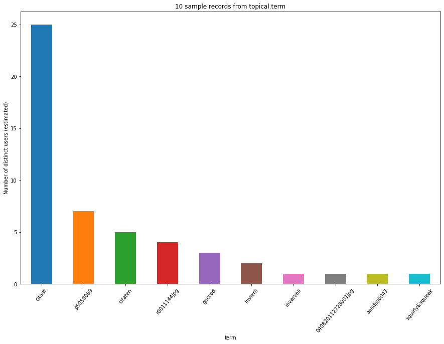
term base
facet = "topical"
base = "term"
samples = 10
Get data from topical.term:
def get_samples(facet: str, base: str, samples: int):
    """Get samples from db"""
    db_query = f"""
        SELECT * FROM {facet}.{base} LIMIT {samples};
    """
    df = db_conn.query(db_query)
    return df
df = get_samples(facet=facet, base=base, samples=samples)
display(df.head())
def list_components(df, facet: str = None, base: str = None):
    """Formatted display of structure components (overlays and bases)"""
    comp = [
        '**Base**',
        '**Overlay(s) (hll metrics)**',
        '**Additional (supplementary base information)**']
    hll_cols = []
    if base is None:
        bases = []
    else:
        bases = [base]
    additional = []
    for col in df.columns:
        if col.endswith("_hll"):
            hll_cols.append(col)
            continue
        if bases is None:
            bases.append(col)
        else:
            if col not in bases:
                additional.append(col)
    display(Markdown(f'### <u>{facet}.{base}</u>'))
    for ix, li in enumerate([bases, hll_cols, additional]):
        if not li:
            continue
        display(Markdown(f'{comp[ix]}: {", ".join([f"*{li_}*" for li_ in li])}'))

list_components(df, facet=facet, base=base)
def get_cardinality(
    facet: str, base: str, metric: str, samples: int):
    """Get cardinality of samples from db"""
    db_query = f"""
    SELECT hll_cardinality({metric})::int, {base}
    FROM {facet}.{base} LIMIT {samples};
    """
    df = db_conn.query(db_query)
    df = df.set_index([base])
    df.sort_values(
        by="hll_cardinality", ascending=False, inplace=True)
    return df
df = get_cardinality(
    metric="user_hll", facet=facet, base=base, samples=samples)
df.head()
def plot_df_bar(
    df: pd.DataFrame, title: str, ylabel: str, xlabel: str):
    """Generate barplot from df"""
    plt.figure(figsize=(15,10))
    cmap = plt.cm.tab10
    colors = cmap(np.arange(len(df)) % cmap.N)
    df["hll_cardinality"].plot.bar(color=colors)
    plt.xticks(rotation=50)
    plt.title(title)
    plt.xlabel(xlabel)
    plt.ylabel(ylabel)
    plt.show()
plot_df_bar(
    df, title=f"{samples} sample records from {facet}.{base}",
    ylabel="Number of distinct users (estimated)", xlabel=f"{base}")
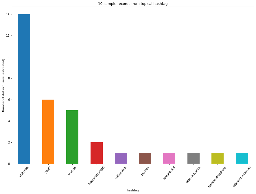
hashtag base
base = "hashtag"
df = get_samples(facet=facet, base=base, samples=samples)
display(df.head())
df = get_cardinality(
    metric="user_hll", facet=facet, base=base, samples=samples)
df.head()
plot_df_bar(
    df, title=f"{samples} sample records from {facet}.{base}",
    ylabel="Number of distinct users (estimated)", xlabel=f"{base}")
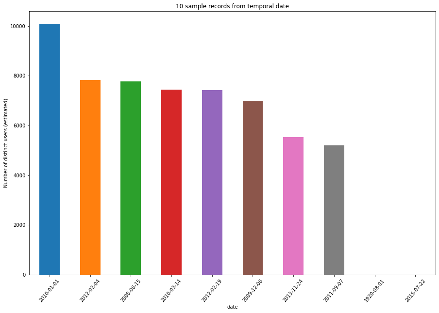
facet = "temporal"
base = "date"
samples = 10
df = get_samples(facet=facet, base=base, samples=samples)
display(df.head())
df = get_cardinality(
    metric="user_hll", facet=facet, base=base, samples=samples)
display(df.head())
plot_df_bar(
    df, title=f"{samples} sample records from {facet}.{base}",
    ylabel="Number of distinct users (estimated)", xlabel=f"{base}")
facet = "spatial"
base = "latlng"
Get sample data for Dresden:
db_query = f"""
    SELECT latitude, longitude, hll_cardinality(post_hll)::int
    FROM {facet}.{base} t1
    WHERE t1.latlng_geom
        && -- intersects
        ST_MakeEnvelope (
         13.46475261, 50.90449772, -- bounding
         14.0876945, 51.24305035, -- box limits (Dresden)
         4326)
"""
df = db_conn.query(db_query)

display(df.head())
Create geoviews point layer:
points_lonlat = gv.Points(
    df,
    kdims=['longitude', 'latitude'], vdims=['hll_cardinality'])
Plot points on map:
def set_active_tool(plot, element):
    """Enable wheel_zoom in bokeh plot by default"""
    plot.state.toolbar.active_scroll = plot.state.tools[0]

hv.Overlay(
    gv.tile_sources.EsriImagery * \
    points_lonlat.opts(
        tools=['hover'],
        size=1+dim('hll_cardinality')*0.1,
        line_color='black',
        line_width=0.1,
        fill_alpha=0.8,
        fill_color='yellow')
    ).opts(
        width=800,
        height=480,
        hooks=[set_active_tool],
        title='Estimate Post Count for distinct yfcc coordinates',
        projection=ccrs.GOOGLE_MERCATOR,
    )