Lecture: Chaos in higher-dimensional systems - Wintersemester 2019/2020
Time/place
 Format: 3+1, i.e. one week with two lectures,
and the following with one lecture and one tutorial session.
 Monday 5. DS (14:50-16:20), BZW/A120
Tuesday 5. DS (14:50-16:20), WIL/A221
The lecture starts on Monday, 14th October 2019.
Audience: Bachelor und Master (Modul Physikalische Vertiefung), Doktoranden, IMPRS
Contents
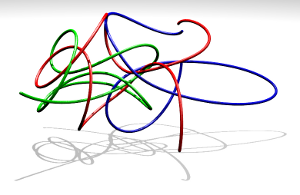
Many physical systems of interest have more than two degrees of freedom which can lead to highly complicated dynamical behavior. Examples are the solar system, atoms and molecules, particle accelerators, or chains of coupled oscillators. In this course we give a general introduction to the dynamics of such higher--dimensional systems. Central for the understanding are invariant objects like fixed points, periodic trajectories, invariant tori, and stable and unstable manifolds. So-called non-linear resonances play a crucial role as they are at the heart of the famous Arnold diffusion, which exclusively occurs in higher-dimensional systems.The course will make use of a combination of rigorous mathematical results (including ideas of their proofs), physicists reasoning (aka hand-waving of different severity) and numerical investigations.
Mailing list
To discuss questions on the lectures and exercise sheets and to exchange ideas a mailing list has been set up.To subscribe, please visit this page.
Do not forget to reply to the automatically generated mail; otherwise the subscription is not activated!
Literature
literature.pdfInformation on Python
German introduction to python/numpy/matplotlib [einfuehrung.pdf, einfuehrung2.pdf].A detailed guide to python and numpy/scipy/matplotlib are the Python Scientific Lecture Notes.
Jupyter notebooks for symbolic computations
To locally start the notebook server run in a konsolejupyter labor
jupyter notebookPoint your web-browser to the given link
http://localhost:8888/?token=9c9d6d828c0c....To create a new notebook, use File/New/Notebook using Python 3. For an example see standard_map.ipynb, which will look as standard_map.html.
Exercises, references, code, ...
All this can be found here (password protected, see first lecture).Last modified: 07 November 2019, 15:54:07, Arnd Bäcker
Computational Physics Group Home.