Tools for Scientific Computation
.
Python rocks
.
Open source is important...
.
https://wwwpub.zih.tu-dresden.de/~baecker/misc/py4science
.
Talk at IIT Madras, Arnd Bäcker, 28th February 2017
Overview - Tasks
Choosing the right tools
Numerical computations
Plotting:
2D graphics
Interactive plots (react on mouse clicks)
3D visualizations
Publication quality plots
Symbolic computations
Application writing
Tools for collaborative work
Choosing the right tools
Basic decision: Closed source vs. Open Source
Eg.: matlab/mathematica?
(+) well established, well tested
(+) good documentation
(+) many toolboxes
(-) expensive
(-) complicated license set-up (does it work in the plane?)
(-) availability at other universities?
(-) running on cluster of CPUs?
(-) ...
Good alternative: python + numpy + scipy + matplotlib + ...
Numerical computations
Classical languages
Fortran
C/C++
Time-consuming to write, runs fast.
High-level languages
Python
Julia ...
Fast(er) to write, may run slower than required.
For speed: if necessary: use Cython/embed C/C++ code.
Important Coding time (your time) vs. running time.
Python - some simple examples
Interactive usage with ipython:
import numpy as np
x = np.linspace(0.0, 1.0, 10)
y = np.sin(x)
print(x)
print(y)
Array operations:
z = x + 5 * y
Python - Useful packages
Numerical computations I
Matrix diagonalization:
import numpy as np
mat = np.random.rand(10, 10)
np.linalg.eigvals(mat)
np.linalg.eig(mat)
Singular value decomposition:
np.linalg.svd(mat)
And (among others):
Solve linear system of equations
QR decomposition
Cholesky decomposition
For even more, see scipy.linalg.
Numerical computations II
Fast Fourier transform:
import numpy as np
from scipy.fftpack import fft
x = np.linspace(0.0, 2.0*np.pi, 100, endpoint=False)
y = np.sin(x)
fft_y = fft(y)
print(fft_y)
Much more, see:
import scipy
help(scipy)
and Scipy Lecture Notes.
Plotting I: 2D graphics, matplotlib
http://matplotlib.org/users/screenshots.html
Example:
ipython --matplotlib

from matplotlib import pyplot as plt

x = np.linspace(0.0, 10.0, 100)
plt.plot(x, np.sin(x), lw=4)
Remarks
Excellent quality for bitmapped output (
.jpg,.png).Good for quick plots
Interactive plots
Output is not of publication quality (IMHO)
Plotting II: 2D graphics, mouse interaction
Code structure:
plt.subplot(111, aspect=1.0)
plt.axis([-1, 1, -1, 1])
plt.xlabel("x")
plt.ylabel("y")

[...]
plt.plot(x_pkt, y_pkt)      # plot something

plt.connect('button_press_event', function_called_on_click)

plt.show()
Examples: spirale.py, kicked_rotor.py
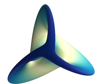
Plotting III: 3D graphics: mayavi
http://code.enthought.com/projects/mayavi/, docu
import numpy as np
from mayavi import mlab

def f(x, y):
    return np.sin(x+y) +  np.sin(2*x - y) + np.cos(3*x+4*y)

def show_surface():
    """Show surface on regularly spaced coordinates."""
    x, y = np.mgrid[-7.:7.05:0.1, -5.:5.05:0.05]
    surface = mlab.surf(x, y, f)
    mlab.outline()
    mlab.axes()
    mlab.show()

show_surface()
Plotting III: 3D graphics: mayavi

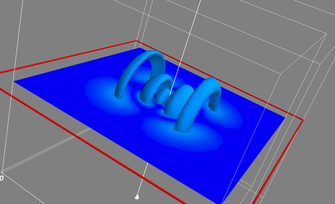
Plotting III: 3D graphics: mayavi
Plotting III: 3D graphics: mayavi
Generate 3D data set for probability density.
Visualize:
mayavi2 -d 5_2_1.vtk -m IsoSurface -m ScalarCutPlane -m Axes -m Outline
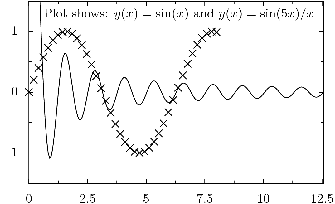
Plotting IV: publication quality plots: pyx
Webpage: http://pyx.sourceforge.net/
import numpy as np
import pyx

x = np.linspace(0.0, 8.0, 40)
y = np.sin(x)

xaxis = pyx.graph.axis.lin(min=0, max=4*np.pi)
yaxis = pyx.graph.axis.lin(min=-1.5, max=1.5)
pgr = pyx.graph.graphxy(width=8, x=xaxis, y=yaxis)
pgr.plot(pyx.graph.data.values(x=x, y=y))
pgr.plot(pyx.graph.data.function("y(x)=sin(5*x)/x", points=200))
pgr.text(0.4, 4.5, r"Plot shows: $y(x) = \sin(x)$ and $y(x)=\sin(5x)/x$")
pgr.writePDFfile("pyx_example")
Plotting IV: publication quality plots: pyx
Webpage: http://pyx.sourceforge.net/
pyx_example.py - result
Plotting IV: publication quality plots: pyx
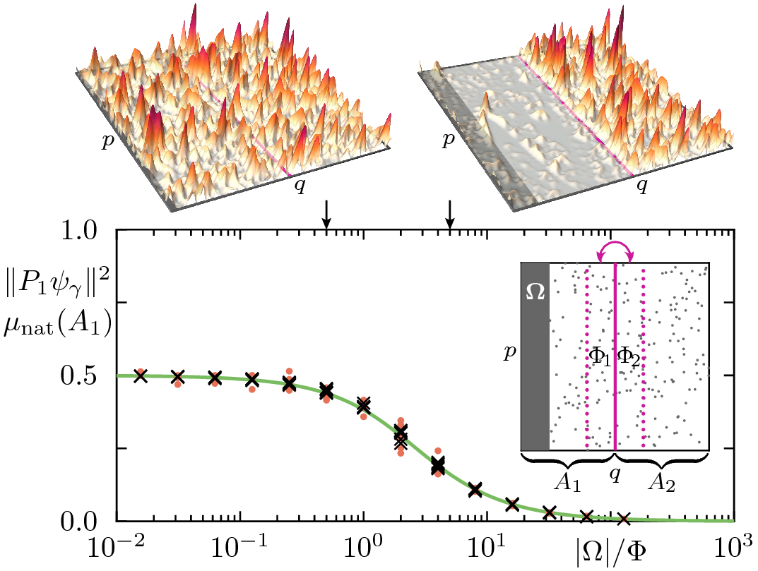
Fig. 1 from: M. J. Körber, A. B. and R. Ketzmerick,
Localization of Chaotic Resonance States due to a Partial Transport Barrier,
Jupyter notebooks
Notebook for python code (and many other languages):
jupyter notebook

Point your browser to ``http://localhost:8888/``.
Example:
%matplotlib inline
import matplotlib.pyplot as plt
import numpy as np

x = np.linspace(0.0, 10.0, 10)
y = np.sin(x)/x

plt.figure()
plt.plot(x, y, 'r')
plt.xlabel('x')
plt.ylabel('y')
plt.show()Symbolic computations - SymPy
http://www.sympy.org, some examples: sympy notebook)
For example:
from sympy import *
init_printing()

x, y, z = symbols('x y z')
a = x**2 - 1
a
a.subs(x, y+1)

a = (x**3-y**3)/(x**2-y**2)
cancel(a)

trigsimp(2*sin(x)**2+3*cos(x)**2)

%matplotlib inline
plot(sin(x)/x, (x, -10, 10))
Application writing
Trait objects can be modified by a GUI, traits_ui_example.py:
from traits.api import HasTraits, Str, Range

class Person(HasTraits):
    first_name = Str("John")
    last_name = Str("Cleese")
    height = Range(0,3.0,1.80)


mr_x = Person()
mr_x.configure_traits(kind="modal")
Examples
iterator
explorator
Collaborative working I: Exchanging files
Instead of dropbox, use
owncloud/nextcloud for:
file exchange
(shared) calenders
note taking (shared documents)
Collaborative working II: git
Version control using git for: code, notes, publications,...
Local usage:
git init
emacs first_file.txt
git add first_file.txt
git commit -m "first file added."
Status, History, differences:
git status
git log
git diff  VersionHashCode
Collaborative usage: Server needed:
gitlab installation of the computing centre (ask them!)
overleaf.com for shared LaTeX documents
Summary
Have a look at:
python+numpy,scipy,matplotlib, ...Comes with batteries included, many tasks already solved...
3D visualization:
mayaviFor publication quality plots:
pyxTools for collaborative work:
owncloud/nextcloud,git,...
Use Open Source whenever possible!
Thanks
Generated using rst2html5 with reveal.js
Some further links
Python Data Analysis Library pandas: Python Data Analysis Library
To install python: Anaconda
A.B.: Computational Physics Education with Python, Computing in Science and Engineering, (2007), 30-33.